Gallager's Sparse Graphs

The series opener ended on an uncomfortable note: Shannon proved in 1948 that near-capacity codes exist in overwhelming abundance, then left no hint of how to decode one. The first real answer arrived remarkably early. In 1960, an MIT doctoral student named Robert Gallager worked out a family of codes with just enough structure to decode and just enough randomness to be good, published the full theory as a 1963 MIT Press monograph, Low-Density Parity-Check Codes, and then watched the field shelve it for thirty years. This page is about what that monograph contained, which turns out to be nearly everything: the codes, the decoder we now call belief propagation, the ensemble method modern coding theory runs on, even computer simulations. Why it was ignored, and the 1993 shock that forced everyone to go back and read it, come at the end.

The LDPC Ensemble: Definition and Construction

Every linear block code is defined by a parity-check matrix $H$: a received word $\mathbf{x}$ is a codeword exactly when $H\mathbf{x}^\mathsf{T} = \mathbf{0}$, and each row of $H$ is one parity equation over a subset of the bits. Gallager’s move is to make $H$ sparse in a very controlled way. An $(n,j,k)$ low-density parity-check code has an $H$ with $n$ columns (one per code bit), exactly $j$ ones in every column (each bit participates in $j$ parity checks), and exactly $k$ ones in every row (each check constrains $k$ bits), with $j$ and $k$ held constant as $n$ grows. That last clause is what “low density” means: the fraction of ones per column, $j/n$, vanishes as $n \to \infty$, so a code of length ten thousand still has only three or four ones in each column.

One notation warning before anything else, because it bites everyone eventually: in Gallager’s $(n,j,k)$, the symbol $k$ is the check degree, the number of bits per parity equation. It is not the number of information bits, despite forty years of $(n,k)$ block-code convention saying otherwise. Modern papers sidestep the collision by writing $d_v$ and $d_c$ for the two degrees; when this series reaches irregular codes, that is the notation it will switch to.

Counting rows: each of the $m$ rows accounts for $k$ ones and each of the $n$ columns for $j$, so $mk = nj$ and $m = nj/k$. The design rate is therefore

$R \;\ge\; 1 - \frac{m}{n} \;=\; 1 - \frac{j}{k},$

with equality when the rows are linearly independent. In practice the ensemble typically carries a few dependent rows, which only makes the true rate slightly higher. A $(3,6)$ code is rate $1/2$, a $(3,4)$ code is rate $1/4$, and so on.

Gallager’s construction of such a matrix is disarmingly simple. Partition $H$ into $j$ horizontal bands, $H = [H_1; H_2; \dots; H_j]$. The first band is a staircase: row $i$ of $H_1$ puts its $k$ ones in columns $(i-1)k+1$ through $ik$, so the $n/k$ rows tile the columns in consecutive blocks. Each remaining band is an independent random column permutation of $H_1$. The bands guarantee the row and column weights exactly; the permutations inject the randomness.

That word “random” points at the methodological move that recurs through everything modern in coding theory. Gallager does not analyze a code. He defines an ensemble, the set of all codes reachable by choosing the permutations at random, and proves that almost every member is good. This is precisely Shannon’s random-coding argument, restricted to a structured family: instead of averaging over all possible codes, almost all of which are undecodable, average over a family every member of which comes with a feasible decoder. Sparsity keeps decoding cheap; the permutations keep the Shannon-style averaging argument alive.

What does sparsity actually buy? Two things, one obvious and one deep. The obvious one: each check involves only $k$ bits and each bit sits in only $j$ checks, so every operation the decoder needs is cheap and local. The deep one: the bipartite graph of a sparse random matrix is locally tree-like. Walk outward from any bit through its checks, to their other bits, to those bits’ other checks, and for the first several hops you almost never revisit a node. On an actual tree, passing local probability messages along the edges computes the exact posterior probability of each bit. Gallager’s decoder runs that computation anyway, on a graph that is only almost a tree, and it works almost exactly. Every result on this page circles back to one of those two purchases.

The Tanner Graph Representation

The single most useful way to look at $H$ is as a bipartite graph, later named after Michael Tanner. Put one variable node on the top row for each of the $n$ code bits (each column of $H$), one check node on the bottom row for each of the $m$ parity equations (each row), and draw an edge between variable $v$ and check $c$ wherever $H$ has a 1. Each variable node has degree $j$, each check node degree $k$, and each check node asserts one equation $\bigoplus_{v \in N(c)} x_v = 0$ over its neighbors.

A deliberately tiny example makes the translation concrete. Take

$H = \begin{pmatrix} 1&1&0&1&0&0 \\ 0&1&1&0&1&0 \\ 1&0&1&0&0&1 \end{pmatrix}, \qquad n=6,\ m=3,$

and read it one row at a time. The first row carries ones in columns 1, 2 and 4, so check $c_1$ ties together bits 1, 2 and 4; the second row gives $c_2$ the bits 2, 3 and 5; the third gives $c_3$ the bits 1, 3 and 6. Those nine ones are exactly the nine edges of the drawing:

From here on it is worth reading every parity-check matrix as a graph, because the decoder does not really operate on a matrix at all: it passes messages along these edges. Do note that this particular example is far too small and too irregular to be a genuine low-density code, since its columns carry only one or two ones apiece and the next section explains why a column weight below three is fatal at scale. It is sized for tracing a decoder by hand, which is exactly what we will do with it shortly.

The graph-theoretic quantity that matters most is the girth: the length of the shortest cycle. In a bipartite graph every cycle alternates sides, so all cycles are even and the girth is at least 4; girth exactly 4 means two variables share two checks, the tightest and most damaging loop, and constructions always avoid it. The drawing above has no such pair, but follow the walk $v_1 \to c_1 \to v_2 \to c_2 \to v_3 \to c_3 \to v_1$ and you close a cycle of length 6, so this little graph has girth 6. Girth measures precisely how locally tree-like the graph is: message passing is exact out to half the girth, and everything beyond is the approximation the decoder lives with.

Minimum Distance of the Ensemble

Why not take $j = 2$ and enjoy the cheapest possible code? Gallager’s Chapter 2 studies minimum distance across the ensemble, and the $j=2$ case is special enough that he gives it its own theorem. His Theorem 2.5 says: for any code in which every bit sits in exactly two checks of $k$ bits each, the minimum distance $D$ is bounded above by a quantity growing only logarithmically in $n$. The proof is a short, beautiful graph argument worth walking through.

Root a tree at bit 1. Since $j = 2$, that bit belongs to exactly two checks, giving two branches from the root. The other $k-1$ bits of each of those checks form tier 1. Each tier-1 bit belongs to exactly one further check (its other check is the one it arrived by), which branches to $k-1$ new bits in tier 2, and so on: tier $m$ contains $2(k-1)^m$ nodes. If all the nodes were distinct bits, the tiers would have to fit inside the code, so $\sum_{i \le m} 2(k-1)^i \le n$, which forces the expansion to fail after

$m \;=\; O\!\left(\frac{\log n}{\log(k-1)}\right)$

tiers: some node must repeat, and a cycle closes at logarithmic depth. Now look at that cycle and mark the check-intersection nodes along it. Each check on the loop contains exactly two of the marked bits. Set the marked bits to 1 and every other bit to 0: every check in the code sees either zero or two ones, an even number either way, so every parity equation is satisfied. That vector is a codeword, and its weight is at most the loop length, which is $O(\log n)$.

A code whose minimum distance grows like $\log n$ is hopeless, so $j = 2$ is out, and every practical LDPC code since has obeyed the rule $j \ge 3$. (The rule has a modern afterlife: irregular codes do admit degree-2 variable nodes, but density evolution caps their fraction through the stability condition, which is this 1963 theorem reborn in analytic clothing. That story belongs to a later page.)

What does $j \ge 3$ buy instead? Linear distance, and Gallager’s Chapter 2 computes exactly how much, by a generating-function argument compact enough to reproduce here. Start with the band construction. A vector satisfies the staircase band $H_1$ exactly when every one of its $n/k$ consecutive blocks of $k$ positions contains an even number of ones. For one block, the polynomial that counts subsets by size while keeping only the even sizes is the standard even-part trick:

$\frac{(1+x)^k + (1-x)^k}{2},$

since adding the two expansions cancels every odd power and doubles every even one. The blocks are disjoint, so the count for the whole band is the $n/k$-th power, and the number of weight-$\ell$ vectors satisfying one band is the coefficient

$N_1(\ell) \;=\; \left[x^\ell\right]\left(\frac{(1+x)^k+(1-x)^k}{2}\right)^{n/k}.$

The other $j-1$ bands are independent random permutations, and a permutation does not change a vector’s weight, so for a fixed weight-$\ell$ vector the probability of satisfying a permuted band is just the fraction of weight-$\ell$ vectors that satisfy a band, $N_1(\ell)/\binom{n}{\ell}$. Multiplying across the $j$ bands and summing over all $\binom{n}{\ell}$ candidate vectors, the ensemble-average number of weight-$\ell$ codewords is

$\mathbb{E}\!\left[N_\ell\right] \;=\; \binom{n}{\ell}\left[\frac{N_1(\ell)}{\binom{n}{\ell}}\right]^{j} \;=\; \binom{n}{\ell}^{\,1-j}\,N_1(\ell)^{\,j}.$

Now go asymptotic. Put $\delta = \ell/n$ and take $\frac{1}{n}\ln(\cdot)$ of everything. The binomial coefficient contributes the binary entropy in nats, $H(\delta) = -\delta\ln\delta - (1-\delta)\ln(1-\delta)$, and the coefficient extraction is a saddle-point (equivalently Chernoff) bound, $\frac{1}{n}\ln N_1(\delta n) \to \mu(\delta) = \min_{s>0}\big[\tfrac{1}{k}\ln\tfrac{(1+s)^k+(1-s)^k}{2} - \delta\ln s\big]$. The result is the distance exponent

$\boxed{\;f(\delta) \;=\; (1-j)\,H(\delta) \;+\; j\,\mu(\delta).\;}$

Read it this way: wherever $f(\delta) < 0$, the expected number of codewords of weight $\delta n$ decays exponentially in $n$, so by Markov’s inequality almost every code in the ensemble has no codeword at that relative weight. The typical minimum-distance ratio $\delta_0 = d_{\min}/n$ is therefore the smallest positive root of $f(\delta) = 0$. Running the computation for several ensembles gives:

$(j,k)$	Rate	$\delta_0 = d_{\min}/n$
$(3,6)$	1/2	0.0227
$(4,8)$	1/2	0.0627
$(5,10)$	1/2	0.0843
$(3,4)$	1/4	0.1122
$(4,6)$	1/3	0.1288

And the $j=2$ case shows up in this analysis too, as an absence: with $j=2$ the exponent satisfies $f(\delta) > 0$ for every $\delta > 0$ (for the $(2,4)$ ensemble, $f(0.001) = +0.0011$, $f(0.01) = +0.0109$, $f(0.1) = +0.1050$, monotonically positive), so there is no root and no linear-distance guarantee at all. That is the analytic shadow of Theorem 2.5’s logarithmic bound, visible in the same plot.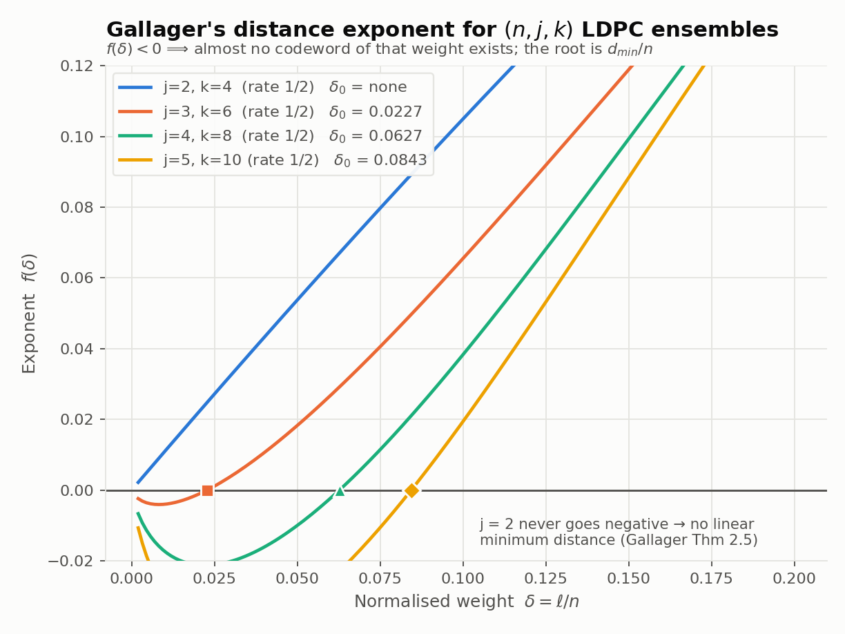

Look at the table once more, because it hides a tension that shapes everything downstream. Increasing $j$ at fixed rate improves the distance ratio dramatically: from 0.023 at $j=3$ to 0.084 at $j=5$. By the distance criterion you should crank $j$ up. Yet every modern design uses $j = 3$ or $4$. The reason is that minimum distance is not what governs the iterative decoder: the noise level at which message passing stops converging, the threshold, gets worse as $j$ rises. Distance-optimal and decoder-optimal point in opposite directions, and 1963’s criterion loses to the decoder’s. Making that threshold computable, so the trade can be settled with numbers rather than folklore, is exactly what the density-evolution page of this series is about.

Bit-Flipping Decoding

Gallager’s simplest decoder is still the right one to understand first, because the sophisticated decoder is this one with probabilities in place of votes. His Algorithm A: compute all the syndromes; if every check passes, stop. Otherwise, for each bit, count how many of its $j$ checks are unsatisfied, flip every bit whose count exceeds a threshold (say more than $j/2$), and repeat. His Algorithm B refines this by making the flip threshold $b$ a parameter that decreases across iterations, so only the most confidently wrong bits get flipped early.

The six-bit code you met as a graph earlier is the right size to watch this happen. Transmit the all-zero codeword and let the channel flip bit 3, so the received word is $\mathbf{r} = (0,0,1,0,0,0)$. Evaluate its three checks, reading each one off the edges leaving that check node:

Check	Bits involved	Sum	Status
$c_1$	1, 2, 4	$0+0+0=0$	satisfied
$c_2$	2, 3, 5	$0+1+0=1$	unsatisfied
$c_3$	1, 3, 6	$0+1+0=1$	unsatisfied

Now count unsatisfied checks per bit: bit 1 touches one failed check, bit 2 one, bit 3 two, bit 4 zero, bits 5 and 6 one each. Bit 3 is the unique maximum. Flip it, re-evaluate, and every check passes: decoded in one iteration.

The intuition to carry out of this example is the engine of everything that follows: an erroneous bit is the only bit common to all the checks it breaks. Errors are localized by the intersection of failed constraints. Bit flipping implements that intersection with hard votes, all-or-nothing, and it works when errors are sparse enough that their footprints do not overlap. Belief propagation, next, is the identical piece of reasoning done with soft, probability-weighted votes, so that a check which is probably telling the truth counts for more than one that is barely sure.

Belief-Propagation Decoding

Section 4.2 of the monograph presents what we now call belief propagation on the Tanner graph, published about twenty years before Pearl gave the algorithm its name in the AI literature. It rests on one lemma.

Gallager’s Lemma 4.1. Given $m$ independent bits where bit $\ell$ equals 1 with probability $P_\ell$,

$\boxed{\;\Pr[\text{an even number of the } m \text{ bits are } 1] \;=\; \frac{1}{2} + \frac{1}{2}\prod_{\ell=1}^{m}\left(1 - 2P_\ell\right).\;}$

The proof is slick enough to give in full. Consider the product $\prod_{\ell=1}^m (1 - P_\ell + P_\ell t)$: expanded in powers of $t$, the coefficient of $t^i$ is exactly $\Pr[\text{exactly } i \text{ ones}]$, since each factor contributes $P_\ell t$ when bit $\ell$ is a one and $1-P_\ell$ when it is a zero. The companion product $\prod_\ell (1 - P_\ell - P_\ell t)$ is identical except that every odd power of $t$ carries a minus sign. Add the two: odd terms cancel, even terms double. Set $t = 1$ and divide by 2. The first product collapses to 1 and the second to $\prod_\ell(1 - 2P_\ell)$, which is the claim.

The right way to internalize the lemma is through the quantity $\varepsilon_\ell \triangleq 1 - 2P_\ell \in [-1,1]$, the soft bit or correlation, $\varepsilon = \mathbb{E}[(-1)^x]$: it is $+1$ for a certain zero, $-1$ for a certain one, and 0 for a coin flip. In this language the lemma says that soft bits multiply across a parity check. One certain input leaves the product’s magnitude alone; one useless input ($\varepsilon = 0$) annihilates it, exactly as it should, since a parity constraint involving one completely unknown bit tells you nothing about the others. That single multiplicative fact is the engine of the whole algorithm.

Now the decoder. Let $P_d$ be the probability that bit $d$ is 1 given only its own channel observation, let $P_{i\ell}$ be the same quantity for the $\ell$-th other bit of the $i$-th check containing $d$, and let $S$ be the event that all $j$ checks on $d$ are satisfied. Gallager’s Theorem 4.1 states:

$\boxed{\;\frac{\Pr[d = 0 \mid \{y\}, S]}{\Pr[d = 1 \mid \{y\}, S]} \;=\; \frac{1 - P_d}{P_d}\;\prod_{i=1}^{j}\;\frac{1 + \prod_{\ell=1}^{k-1}\left(1 - 2P_{i\ell}\right)}{1 - \prod_{\ell=1}^{k-1}\left(1 - 2P_{i\ell}\right)}.\;}$

Read it as: posterior odds equals channel odds times a product of $j$ check contributions, each of which comes straight out of Lemma 4.1. And notice the upper limit of the inner product: $\ell$ runs to $k-1$, over the other bits of the check, never including $d$ itself. Each check reports what the rest of its bits imply about $d$, uncontaminated by $d$‘s own opinion. This is the extrinsic principle, and it is sitting right there in Gallager’s 1963 formula; the same principle resurfaces, rediscovered, as the heart of turbo decoding thirty years later.

The proof takes four sentences of Bayes and one crucial assumption. Split the observation of bit $d$ from everything else:

$\frac{\Pr[d=0\mid \{y\},S]}{\Pr[d=1\mid \{y\},S]} \;=\; \frac{\Pr[d=0\mid y_d]}{\Pr[d=1\mid y_d]}\cdot\frac{\Pr[S\mid d=0,\{y\}]}{\Pr[S\mid d=1,\{y\}]}.$

The first factor is the channel’s own opinion, $(1-P_d)/P_d$. For the second, consider check $i$, which contains $d$ plus $k-1$ other bits. If $d = 0$, the check is satisfied exactly when the other $k-1$ bits hold an even number of ones; if $d = 1$, exactly when they hold an odd number. Lemma 4.1 gives those two probabilities as $\tfrac12 \pm \tfrac12\prod_{\ell=1}^{k-1}(1-2P_{i\ell})$. Finally, under the tree hypothesis the $j$ checks on $d$ involve disjoint sets of other bits, so the event $S$ that all of them are satisfied factorizes into a product of the $j$ per-check ratios. Multiply the factors and the theorem follows.

Mark exactly where the tree assumption entered: in the single word “factorizes.” The proof claimed the $j$ checks are independent given $d$, which holds precisely when their other bits are disjoint and themselves independent, which is what a tree guarantees. If two checks were linked through a short path elsewhere in the graph, that is a cycle, and the factorization is invalid. Gallager knew it and said so, in a footnote: if some linear combination of checks not containing $d$ yields a check involving only tier-1 digits, independence fails. That is a cycle, described before the graph language for it existed. His tree figure makes the positive statement explicit: iterate the formula, feeding each $P_{i\ell}$ the posterior computed for that bit in the previous round (excluding the contribution that arrived through check $i$, extrinsic again), and the result is exact for as long as the depth-$m$ neighborhood of $d$ remains a tree. That footnote is the entire gap between exact inference and the heuristic that happens to work, and the modern analysis of LDPC codes amounts to measuring it.

The Sum-Product Algorithm in LLR Form

Nobody implements Theorem 4.1 in probability coordinates; products of odds ratios are numerically miserable. The modern form substitutes the log-likelihood ratio $L = \ln\frac{1-P}{P}$, under which $1 - 2P = \tanh(L/2)$, and the theorem splits into two alternating message rules on the Tanner graph.

The variable-to-check message sums the other opinions about the bit:

$L_{v \to c} \;=\; L_{\text{ch}}(v) \;+\; \sum_{c' \in N(v)\setminus\{c\}} L_{c' \to v},$

which is just the fact that independent evidence about the same quantity adds in the log domain; it is Theorem 4.1’s outer product of $j$ factors, taken to $j-1$ of them and pushed through the logarithm. The check-to-variable message is Lemma 4.1 in disguise, the tanh rule:

$\tanh\!\left(\frac{L_{c \to v}}{2}\right) \;=\; \prod_{v' \in N(c)\setminus\{v\}} \tanh\!\left(\frac{L_{v' \to c}}{2}\right),$

soft bits multiplying across the check, with the target bit excluded, and inverted via $L_{c\to v} = 2\,\mathrm{artanh}(\prod \tanh(L_{v'\to c}/2))$. The final decision for each bit uses everything, including the bit’s own channel value, with no exclusion:

$L(v) = L_{\text{ch}}(v) + \sum_{c \in N(v)} L_{c \to v}, \qquad \hat{x}_v = \tfrac{1}{2}\left(1 - \mathrm{sign}\, L(v)\right).$

The decoder stops when $H\hat{\mathbf{x}}^\mathsf{T} = \mathbf{0}$, or after a maximum iteration count. That syndrome test is a genuine success indicator: when the estimate satisfies every check, the decoder knows it has landed on a codeword (very occasionally the wrong one, but a codeword), a self-awareness that turbo decoders turn out to lack entirely. And the iteration cap is not just an engineering budget. On a graph with cycles, more iterations do not always help: the messages can oscillate, or converge to a fixed point that is not a codeword and never will be, so past a few dozen iterations you are usually burning power to re-confirm a failure. Cap the count, and trust the syndrome test to say when you have won.

The Min-Sum Approximation and Update Scheduling

The tanh rule is the expensive part of the decoder: transcendental functions on every edge, every iteration. But notice that $\tanh$ saturates quickly, so the product $\prod \tanh(L_{v'}/2)$ is dominated by its smallest-magnitude factor; the near-saturated large inputs contribute sign but hardly any attenuation. Keeping only the dominant term gives the min-sum approximation:

$L_{c\to v} \;\approx\; \left(\prod_{v'} \mathrm{sign}\, L_{v'\to c}\right)\cdot \min_{v'} \left|L_{v'\to c}\right|,$

signs multiply, and the magnitude is simply the least confident input. Comparisons and additions only; no multipliers, no lookup tables. This is what hardware overwhelmingly implements.

But check it numerically before trusting it. Take incoming LLRs $\{+2.0,\ -1.5,\ +3.0\}$. The exact rule gives $2\,\mathrm{artanh}\big(\tanh(1.0)\cdot\tanh(-0.75)\cdot\tanh(1.5)\big) = 2\,\mathrm{artanh}(0.7616 \times (-0.6351) \times 0.9051) = 2\,\mathrm{artanh}(-0.4378) = -0.939$. Min-sum gives sign negative, magnitude $\min(2.0, 1.5, 3.0) = 1.5$, so $-1.5$: the right sign, but a magnitude 60% too confident, because the approximation discards the attenuation every other factor contributes. Treating min-sum as interchangeable with true belief propagation is a standard mistake, and uncorrected it costs several tenths of a dB. The fixes are cheap: normalized min-sum scales the magnitude by $\alpha \approx 0.75$ (here $0.75 \times 1.5 = 1.125$, much closer to $0.939$), and offset min-sum subtracts $\beta \approx 0.15$ with clipping at zero. The pattern is worth filing away: a max-style approximation that systematically over-trusts, healed by a scaling factor near 0.75, is exactly the relationship Max-Log-MAP bears to log-MAP in turbo decoding. Same mathematics, same fix, two literatures.

That claim is easy to test rather than take on faith, and simulating a rate-1/2 regular code at $n = 1008$ bears it out precisely: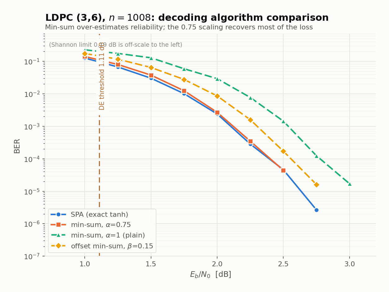

The ordering is exactly what the arithmetic predicted. Uncorrected min-sum pays about half a decibel for its overconfidence, the offset correction takes back roughly half of that, and the single multiplication by $\alpha = 0.75$ recovers nearly all of it: at high SNR the normalized curve is indistinguishable from exact belief propagation, while costing only comparisons and adds. That is the entire reason hardware ships min-sum rather than the tanh rule.

One decision remains: the order in which messages update, the schedule. Flooding updates every check node, then every variable node, in lockstep; it is maximally parallel and is the schedule all the theory assumes. Layered (row-serial) scheduling processes the check rows in groups, letting each group use the freshly updated variable messages immediately; the newer information propagates within an iteration instead of waiting for the next one, and in practice the decoder converges in about half the iterations. Layered is the default in hardware for exactly that reason. Smarter dynamic schedules that prioritize the least-converged messages do better still, at the price of adaptive control logic.

Historical Remarks

Step back and tally what the monograph established. Chapter 2: minimum distance linear in $n$ for $j \ge 3$, with the constant $\delta(j,k)$ tabulated, and the logarithmic ceiling for $j = 2$. Chapter 3: a Chernoff-bound analysis showing the ensemble’s error probability under maximum-likelihood decoding decays exponentially in $n$ at any rate below a computable limit, plus a limitation still quoted today: with bounded check degree $k$, low-density codes cannot quite achieve capacity, though the gap vanishes exponentially fast in $k$ (thirty-eight years later, Richardson, Shokrollahi, and Urbanke would open their landmark paper by restating this as their Theorem 1). Chapter 4: the bit-flipping decoders, the probabilistic decoder with Lemma 4.1 and Theorem 4.1, the extrinsic exclusion, the tree condition for exactness, and an analysis of the iterative decoder’s error probability. Chapter 6: actual computer simulations on binary symmetric, Gaussian, and Rayleigh fading channels. In 1963.

So: good codes, a linear-time iterative decoder, the ensemble method, the extrinsic principle, and simulation evidence, all in print by 1963. Why did the field walk away for thirty years? Because the codes needed block lengths in the thousands and dozens of iterations of floating-point message passing per block, and in 1963 that was not merely expensive for a receiver; it was inconceivable. A single decode was a serious mainframe computation, and a receiver must do it millions of times per second on a power budget. Meanwhile algebraic codes fit the hardware of the era: a Reed-Solomon code concatenated with a convolutional code could be decoded with shift registers and modest logic, performed respectably, and flew on real spacecraft. Concatenated coding became the standard, and Gallager’s monograph settled into the library stacks as a beautiful dead end. The timing of the rediscovery is the tell: MacKay and Neal revived the codes in 1996, three years after a conference paper out of France demonstrated, to general disbelief, that iterative decoding of another code family reached within a fraction of a dB of the Shannon limit. Only then did it become urgent to ask whether anyone had thought of iterative decoding before. Someone had, in full, three decades earlier.

Check Yourself

1. Why must every bit participate in at least three checks? What exactly goes wrong at $j = 2$?
2. Why does the check-node update multiply while the variable-node update adds?
3. In the proof of Gallager’s Theorem 4.1, exactly where does the tree assumption enter, and what breaks on a graph with cycles?
4. Why is the min-sum output systematically overconfident, and what is the fix?
5. Why should an LDPC decoder cap its iteration count rather than run until convergence, and what stopping test should it use?
6. In Gallager’s $(n,j,k)$ notation, what is $k$, and why is the notation dangerous?

Answers

1. At $j=2$, expanding the code as a tree from any bit forces a cycle to close within $O(\log n)$ tiers, and setting the cycle’s check-intersection bits to 1 produces a valid codeword of weight $O(\log n)$: minimum distance grows only logarithmically (Theorem 2.5). For $j \ge 3$ the distance exponent $f(\delta) = (1-j)H(\delta) + j\mu(\delta)$ has a positive root $\delta_0$, so typical minimum distance grows linearly in $n$.

2. A check node constrains the XOR of its bits, and by Lemma 4.1 the soft bit $\varepsilon = 1-2P = \tanh(L/2)$ of an XOR is the product of the individual soft bits. A variable node combines independent evidence about the same bit, and independent log-likelihood evidence adds.

3. It enters when the event “all $j$ checks on $d$ are satisfied” is factorized into per-check probabilities, which requires the $j$ checks to involve disjoint, independent sets of other bits: true on a tree. A cycle makes two checks share information, the factorization fails, and the computed posterior becomes an approximation (Gallager’s own footnote to the theorem).

4. Min-sum keeps only the smallest-magnitude factor of the tanh product, discarding the attenuation every other factor contributes, so its magnitude is always an overestimate ($-1.5$ against the exact $-0.939$ in the worked example, about 60% too confident). Fix with normalized min-sum ($\alpha \approx 0.75$) or offset min-sum ($\beta \approx 0.15$, clipped at zero).

5. On a graph with cycles, belief propagation can oscillate or converge to a non-codeword fixed point, so extra iterations may only re-confirm a failure. Cap the count and stop early when $H\hat{\mathbf{x}}^\mathsf{T} = \mathbf{0}$: the syndrome test is a genuine success indicator.

6. $k$ is the check degree, the row weight of $H$, not the number of information bits of standard $(n,k)$ block-code notation; the rate is $1 - j/k$, so misreading $k$ corrupts every rate calculation. Modern notation writes $d_v$ and $d_c$ to avoid the collision.

Where This Leaves Us

Gallager’s 1963 monograph answered Shannon’s challenge in nearly complete form: sparse random ensembles with provably linear distance for $j \ge 3$, a message-passing decoder that is exact on trees and excellent on the locally tree-like graphs sparsity provides, the extrinsic principle baked into a product that pointedly runs to $k-1$, and simulations to show it all worked. The field shelved it because 1963 hardware could not conceivably run it. The revival, when it came, did not come from anyone rereading the monograph. It came from a 1993 conference talk by two French engineers whose claimed results sat so close to the Shannon limit that reviewers assumed a measurement error, and whose iterative decoder turned out, on inspection, to be passing extrinsic information between two component decoders in exactly the spirit of Gallager’s product to $k-1$. That story, and the code that turned the whole field around, is next: The Turbo Shock of 1993.