The Turbo Shock of 1993

When we left Gallager’s sparse graphs, his iterative decoder had gone to sleep in a 1963 monograph, and the field had settled into a comfortable pessimism. By the early 1990s the working belief was that the last two decibels separating practical codes from Shannon’s promise could only be bought with exponentially growing complexity: longer constraint lengths, bigger trellises, decoders that doubled in cost for every fraction of a decibel gained. Then, at the ICC conference in Geneva in May 1993, three researchers from a French telecommunications school presented a seven-page paper claiming to reach within half a decibel of the Shannon limit using two small convolutional codes and a scrambler. The claim was so far ahead of everything else that several reviewers assumed it was a measurement error. It was not. This page walks through what Berrou, Glavieux and Thitimajshima actually built: the encoder, the full decoder derivation, and the worked example that reveals which inputs a turbo code actually has to fear.

Background and Motivation

To feel the shock, you need the 1992 baseline. The workhorse of deep-space and satellite communication was the convolutional code decoded by the Viterbi algorithm, whose complexity grows as $2^{K-1}$ in the constraint length $K$; practical decoders topped out around $K = 9$. The most powerful deployed system, the CCSDS standard, concatenated a Reed-Solomon outer code with a convolutional inner code and still sat roughly 2 to 3 dB from capacity. Everyone knew Shannon’s theorem promised more, and the opener explained why his proof gave no construction: random codes achieve capacity but cannot be decoded. The consensus was that this gap was structural.

Berrou’s paper reported a bit error rate of $10^{-5}$ at $E_b/N_0 = 0.7$ dB for a rate-1/2 code. The Shannon limit for rate-1/2 binary signalling sits near 0.2 dB, so the gap to capacity was about half a decibel, an order of magnitude closer than anything in deployment. And the decoder was not exponential in anything: it was two small trellis decoders taking turns.

The paper opens with a structural observation that motivates the whole construction. Compare a non-systematic convolutional (NSC) code with a systematic code of the same memory. At high SNR the NSC code wins: its free distance is better. At low SNR the ordering generally reverses, because a systematic code transmits the information bits in the clear and the decoder gets to observe them directly. Berrou’s insight is that a recursive systematic convolutional (RSC) code captures both virtues at once. It is systematic, so every information bit has a direct channel observation, which an iterative decoder turns out to need. And it has the same distance spectrum as its parent NSC code, because the two encoders generate exactly the same set of codewords; only the mapping from inputs to codewords differs. That last sentence sounds like a technicality. Hold onto it, because by the end of this page it will look like the most consequential fact in the paper, and the next page will prove it is.

The Encoder: Parallel Concatenation via an Interleaver

Shannon showed that long random codes are good; the whole problem is decoding them. Berrou’s construction sidesteps the problem rather than solving it. Take two simple rate-1/2 RSC encoders. Feed the information bits $d_k$ to the first one directly, and to the second one after scrambling them with a long pseudo-random interleaver $\pi$. Transmit the information bits once, plus the parity from both encoders:

One systematic stream plus two parity streams makes the concatenation naturally rate 1/3. Berrou punctures the two parity streams alternately (transmit $Y1_k$ on even $k$, $Y2_k$ on odd $k$) to reach rate 1/2 overall; in his accounting each constituent code then operates at rate 2/3. Notice what is not transmitted: the second encoder’s systematic output. It would be a permutation of bits already sent, zero new information and pure rate loss, so it is simply discarded.

The interleaver is the heart of the scheme, and there are two ways to see why, both worth holding in your head at once. The first view is randomness: the overall code has block length $3N$ where $N$ is the interleaver length, and Berrou used $N = 65536$. A code that long, built randomly, would approach capacity by Shannon’s own argument. The interleaver is the injected randomness, and, crucially, it costs the decoder nothing, because the decoder never confronts the long code as a whole. It only ever decodes the two small constituent codes on their own trellises. The second view is decorrelation: if some input pattern happens to produce low-weight parity out of encoder 1, the interleaver makes it overwhelmingly likely that the permuted pattern produces high-weight parity out of encoder 2. Inputs that are bad for one encoder are good for the other. The worked example at the end of this page shows exactly which patterns can defeat this protection, and Gallager would have recognized the spirit immediately: build global structure from local pieces, and let randomness do the heavy lifting.

The constituent encoder deserves a closer look, because “recursive” is doing more work than it appears to. Start from an NSC code with generator polynomials $G_1, G_2$. Convert it to RSC form by feeding the output of one generator back into the input and making the information bit itself the first output:

$a_k = d_k \oplus \sum_{i=1}^{K-1} \gamma_i\, a_{k-i} \pmod 2, \qquad X_k = d_k, \qquad Y_k = \sum_{i=0}^{K-1} g_{2i}\, a_{k-i} \pmod 2$

The shift register now stores the fed-back sequence $a_k$, not the raw input $d_k$. That is the entire difference between the recursive and nonrecursive encoders, and it changes everything. Berrou’s code has $K = 5$ (memory 4), feedback generator $G_1 = 37_8 = 1+D+D^2+D^3+D^4$ and feedforward generator $G_2 = 21_8 = 1+D^4$, giving the transfer function

$G(D) = \left[\, 1, \;\; \frac{1+D^4}{1+D+D^2+D^3+D^4} \,\right].$

Look at that second entry: the feedback polynomial sits in the denominator, so the parity response to a single input 1 is a division of polynomials, and the impulse response is infinite. A nonrecursive encoder forgets a lone input bit after $K$ steps; a recursive encoder never does. File that fact away. The worked example below turns it into the property that makes the whole construction stand up.

The BCJR Decoding Algorithm

The Viterbi algorithm finds the single most likely sequence through the trellis and outputs hard bits. That is exactly the wrong tool here, because an iterative decoder needs, for each individual bit, a soft measure of reliability that it can hand to its partner. What we need is the symbol-by-symbol maximum a posteriori (MAP) decoder: for each bit $d_k$, compute the posterior probability given the entire received block. The algorithm that does this on a trellis is the BCJR algorithm of Bahl, Cocke, Jelinek and Raviv, published in 1974 and largely ignored for two decades because it was more expensive than Viterbi for no gain in hard-decision performance. Berrou calls it “the modified Bahl et al. algorithm”; his contribution is adapting it to RSC codes and, crucially, extracting from its output the piece that is safe to pass between decoders.

One convention note before the formulas, because it bites everyone who reads the original paper: Berrou defines his log-likelihood ratio as $\Lambda(d_k) = \ln \Pr[d_k=1\,|\,\cdot\,]/\Pr[d_k=0\,|\,\cdot\,]$, with the 1-hypothesis on top. These notes use the opposite convention, 0 on top, which flips every sign. Always check the convention before comparing formulas across papers.

BCJR runs on the trellis of one constituent code and is built from four quantities:

Symbol	Name	Meaning	Recursion
$\gamma_k(s',s)$	branch metric	likelihood of the transition $s' \to s$ at time $k$	$\gamma_k(s',s) = \Pr[d_k]\cdot p(\mathbf{y}_k \mid \mathbf{x}_k(s',s))$
$\alpha_k(s)$	forward metric	$\Pr[S_k=s,\ \mathbf{y}_1^k]$	$\alpha_k(s) = \sum_{s'} \alpha_{k-1}(s')\,\gamma_k(s',s)$
$\beta_k(s)$	backward metric	$p(\mathbf{y}_{k+1}^N \mid S_k=s)$	$\beta_k(s) = \sum_{s'} \beta_{k+1}(s')\,\gamma_{k+1}(s,s')$
$L(d_k)$	output LLR	log ratio of posteriors	combination of the three above

Rather than quote these, let us derive them; the derivation is short and every step of the iterative decoder falls out of it.

Start from the joint quantity that a trellis makes natural. For a transition $s' \to s$ at time $k$, define $\sigma_k(s',s) \triangleq \Pr[S_{k-1}=s',\, S_k=s,\, \mathbf{y}_1^N]$: the probability of that particular transition together with the entire received block. Because the information bit $d_k$ is determined by which transition was taken, summing $\sigma_k$ over all transitions carrying $d_k = b$ gives $\Pr[d_k=b,\ \mathbf{y}_1^N]$, and the posterior LLR is

$L(d_k) = \ln\frac{\sum_{(s',s):\,d_k=0}\sigma_k(s',s)}{\sum_{(s',s):\,d_k=1}\sigma_k(s',s)}.$

Now split the observations into past, present and future, $\mathbf{y}_1^N = (\mathbf{y}_1^{k-1},\ \mathbf{y}_k,\ \mathbf{y}_{k+1}^N)$, and factorize:

$\sigma_k(s',s) = \underbrace{\Pr\!\left[S_{k-1}=s',\mathbf{y}_1^{k-1}\right]}_{\alpha_{k-1}(s')}\cdot \underbrace{\Pr\!\left[S_k=s,\mathbf{y}_k \mid S_{k-1}=s'\right]}_{\gamma_k(s',s)}\cdot \underbrace{p\!\left(\mathbf{y}_{k+1}^N \mid S_k=s\right)}_{\beta_k(s)}$

This factorization is exact, and it is exactly where the trellis structure earns its keep. Two conditional-independence facts justify it: given the state $S_{k-1}=s'$, the present transition is independent of the past observations, so the middle factor needs no further conditioning; and given $S_k=s$, the future observations are independent of everything earlier, so the last factor is a clean conditional. The state is a sufficient summary of history. This is the Markov property doing for the trellis what the cycle-free assumption did for Gallager’s graphs.

The recursions now write themselves. Expanding $\alpha_k(s)$ by conditioning on the previous state gives the forward sweep $\alpha_k(s) = \sum_{s'}\alpha_{k-1}(s')\,\gamma_k(s',s)$, initialized by the known starting state: $\alpha_0(0)=1$, $\alpha_0(s)=0$ otherwise. Symmetrically, the backward sweep is $\beta_{k-1}(s') = \sum_s \gamma_k(s',s)\,\beta_k(s)$. Its initialization depends on termination: if the trellis is driven back to the zero state at the end of the block, $\beta_N(0)=1$ and zero elsewhere; if it is not terminated (a common situation for the second constituent encoder, for reasons the worked example makes clear), you must admit ignorance and set $\beta_N(s)$ uniform over all states, a small but genuine loss.

What remains is the branch metric, and here is where the physics of the channel enters. Factor $\gamma_k$ into an a priori part and a channel part: $\gamma_k(s',s) = \Pr[d_k]\cdot p(\mathbf{y}_k \mid \mathbf{x}_k(s',s))$. For a rate-1/2 systematic code over the binary-input AWGN channel, write the received pair as $\mathbf{y}_k = (y^s_k, y^p_k)$, the transmitted BPSK pair as $\mathbf{x}_k = (x^s_k, x^p_k)$ with $x \in \{\pm1\}$, amplitude $a$ and noise variance $\sigma^2$. The Gaussian density contributes $\exp(-[(y^s_k - a x^s_k)^2 + (y^p_k - a x^p_k)^2]/2\sigma^2)$. Expand the squares: the $y^2$ terms and the $a^2 x^2 = a^2$ terms are identical for every hypothesis, so they cancel in the ratio $L(d_k)$ and can be dropped, leaving only the cross terms:

$\gamma_k(s',s) \;\propto\; \Pr[d_k]\cdot \exp\!\left(\tfrac{1}{2}L_c\, y^s_k x^s_k + \tfrac{1}{2}L_c\, y^p_k x^p_k\right), \qquad L_c \triangleq \frac{2a}{\sigma^2}.$

The constant $L_c$ is the channel reliability: how much one channel observation is worth, in LLR units. Finally express the a priori factor through the incoming LLR $L_a$. Since $\Pr[d_k=0]/\Pr[d_k=1] = e^{L_a}$ and the systematic symbol is $x^s_k = 1-2d_k = \pm 1$, a line of algebra gives $\Pr[d_k] \propto e^{x^s_k L_a/2}$ (the omitted prefactor is common to both hypotheses and cancels). Collecting everything:

$\boxed{\;\gamma_k(s',s)\;\propto\;\exp\!\left(\tfrac{1}{2}\,x^s_k\!\left[L_c\,y^s_k + L_a(d_k)\right] \;+\; \tfrac{1}{2}L_c\,y^p_k\, x^p_k\right)\;}$

Read the two exponents. The first depends on the transition only through the bit $d_k$ it carries; it is identical for every branch with the same information bit. The second depends on the parity symbol, which genuinely varies from branch to branch. That structural split is about to become the single most important formula on this page.

The Extrinsic-Information Decomposition

Because the first exponential in the boxed branch metric is the same for every transition with the same $d_k$, we can peel it off. Define the parity-only branch metric $\tilde\gamma_k(s',s) \triangleq \exp(\tfrac{1}{2}L_c\,y^p_k\,x^p_k(s',s))$, so that $\gamma_k = e^{\frac{1}{2}x^s_k[L_c y^s_k + L_a]}\cdot\tilde\gamma_k$. Substitute into the LLR. In the numerator, every term has $d_k=0$ and hence $x^s_k=+1$; in the denominator, $x^s_k=-1$. The common factor pulls straight out of each sum:

$L(d_k) = \ln\frac{e^{+\frac12[L_c y^s_k + L_a]}\sum_{d_k=0}\alpha_{k-1}\,\tilde\gamma_k\,\beta_k}{e^{-\frac12[L_c y^s_k + L_a]}\sum_{d_k=1}\alpha_{k-1}\,\tilde\gamma_k\,\beta_k}$

and the logarithm splits it into three additive pieces:

$\boxed{\;\underbrace{L(d_k)}_{\text{a posteriori}} \;=\; \underbrace{L_c\, y_k^{s}}_{\text{channel observation of bit } k} \;+\; \underbrace{L_a(d_k)}_{\text{a priori, from the other decoder}} \;+\; \underbrace{L_e(d_k)}_{\text{extrinsic}}\;}$

where $L_e(d_k) \triangleq \ln\left(\sum_{d_k=0}\alpha_{k-1}\tilde\gamma_k\beta_k \,/\, \sum_{d_k=1}\alpha_{k-1}\tilde\gamma_k\beta_k\right)$ is built from the parity-only metrics. This is not an assertion; we have just proved it. And notice what $L_e$ does not contain: no $y^s_k$, and no $L_a(d_k)$. It is what the decoder learned about bit $k$ from the parity constraints binding it to the other bits, which is to say, genuinely new information the other decoder does not already have. Berrou calls it the extrinsic information, and in practice you extract it by subtraction: $L_e = L - L_c y^s_k - L_a$.

Why does this matter so much? Suppose you skipped the subtraction and passed the full posterior $L(d_k)$ from decoder 1 to decoder 2 (this is, incidentally, the classic turbo implementation bug). Decoder 2 would receive back its own prior opinion $L_a$, dressed up as fresh evidence. It would reinforce that opinion, pass the reinforced version back, and the loop would converge, confidently, to whatever it happened to believe first. The system becomes a rumor mill: two decoders congratulating each other on agreeing, with the agreement anchored to nothing. The observable symptom is distinctive: the BER improves for two or three iterations and then gets worse. The extrinsic rule is the only thing preventing this positive feedback, and if the idea feels familiar, it should: it is precisely the discipline built into Gallager’s 1963 update rule, where a message sent along an edge deliberately excludes the information that arrived along that same edge. Berrou reinvented the principle, apparently unaware of the precedent, thirty years later.

One honest caveat. The independence of $L_e$ from $L_a(d_k)$ is exact only at time $k$ directly; the metrics $\alpha_{k-1}$ and $\beta_k$ were themselves computed by recursions that touched bit $k$‘s prior through other paths. On a cycle-free graph the independence would be perfect; on a turbo code’s graph (which has cycles, closed through the interleaver) a residual correlation survives. This is why iterative turbo decoding is not exactly maximum-likelihood, and it is why the damping fix described below earns its keep.

Berrou devotes a full section of the paper to the statistics of the extrinsic values, and his Figure 6 records an observation that looks minor and turns out to be prophetic: the histogram of the extrinsic quantity starts out visibly non-Gaussian at the first iteration and converges toward a clean Gaussian with mean $\pm 1$ as the iterations proceed. Six years later that empirical remark became the foundation of EXIT-chart analysis, a story for a later page.

Log-Domain Implementation and the Max-Log-MAP Approximation

As written, the recursions multiply probabilities across a block of $N = 65536$ symbols, which underflows any floating-point format long before the end of the sweep. The fix is the same one every probabilistic algorithm eventually adopts: work with logarithms. Let $\bar\alpha_k = \ln\alpha_k$, $\bar\beta_k = \ln\beta_k$, $\Gamma_k = \ln\gamma_k$. Products become sums, but sums become log-sums-of-exponentials:

$\bar\alpha_k(s) = \ln\sum_{s'} e^{\bar\alpha_{k-1}(s')+\Gamma_k(s',s)} = \operatorname*{max^*}_{s'}\left[\bar\alpha_{k-1}(s')+\Gamma_k(s',s)\right]$

where the two-argument operator is

$\max{}^*(x_1,x_2) \triangleq \ln\left(e^{x_1}+e^{x_2}\right) = \max(x_1,x_2) + \ln\left(1+e^{-|x_1-x_2|}\right).$

The identity takes one line to prove: factor $e^{\max(x_1,x_2)}$ out of the sum and what remains inside the logarithm is $1+e^{-|x_1-x_2|}$. The operator is associative and commutative, so longer sums fold pairwise. The practical miracle is that the correction term $\ln(1+e^{-|\Delta|})$ is a one-dimensional function of the gap $|\Delta|$: in hardware it is an eight-entry lookup table, which is the entire reason exact log-MAP decoding is affordable. Even in the log domain the metrics need per-step normalization (subtract $\max_s \bar\alpha_k(s)$ from every state); since $L(d_k)$ is a difference, any constant common to all states cancels exactly. The output LLR becomes a difference of two $\max^*$ trees, one over the $d_k=0$ branches and one over the $d_k=1$ branches. One more property is worth noting because it will matter when this series reaches the 5G throughput wars: $\beta$ cannot start until the whole block has arrived, so BCJR is inherently non-causal and serial in a way Viterbi is not.

Max-Log-MAP is the simplification everyone actually ships: drop the correction term, so $\max^*$ becomes plain $\max$. This is equivalent to keeping only the single best path through each half of the trellis, a kind of soft Viterbi. It costs roughly 0.3 to 0.5 dB, and it has a systematic bias: by ignoring all but the best path, it overestimates the reliability of its own conclusions. The standard remedy is to scale the extrinsic output by a factor of about 0.7 before passing it on. If you have read the LDPC entry, this should ring a loud bell: the min-sum approximation to Gallager’s check-node rule has exactly the same failure (keeping only the dominant term overstates confidence) and exactly the same fix (scale the message down by a constant near 0.75). This is not a coincidence and it is worth stating as a series thread: max-only approximations to soft-sum computations are systematically overconfident, and a single scalar damping factor recovers most of the loss. We will meet the phenomenon again.

Iterative Decoding and Extrinsic Scaling

The pieces now assemble into the machine. Each constituent decoder is a soft-in soft-out MAP module: it consumes the channel observations of its own parity stream, the systematic observations, and an a priori LLR per bit supplied by the other decoder, and it produces an extrinsic LLR per bit.

One iteration is one pass through DEC 1 followed by DEC 2. Decoder 1’s extrinsic output, interleaved, becomes decoder 2’s a priori input; decoder 2’s extrinsic output, de-interleaved, comes back as decoder 1’s prior for the next round. The loop starts with $L_{a1} = 0$ (no prior knowledge), and after the final iteration you hard-decide each bit from decoder 2’s full posterior $L(d_k)$, de-interleaved. Berrou ran up to 18 iterations; his Figure 5 shows the characteristic diminishing returns, with most of the gain arriving by iteration 6 to 8 and the curves nearly superimposed past 12. That saturation is worth internalizing as its own lesson: more iterations do not always help, and without further precautions they can actively hurt. A fixed iteration count, a CRC-based early stop, or a cross-entropy convergence test are the standard termination rules.

Simulating a rate-1/3 turbo code with a 1024-bit interleaver and exact log-MAP decoding reproduces that behavior directly: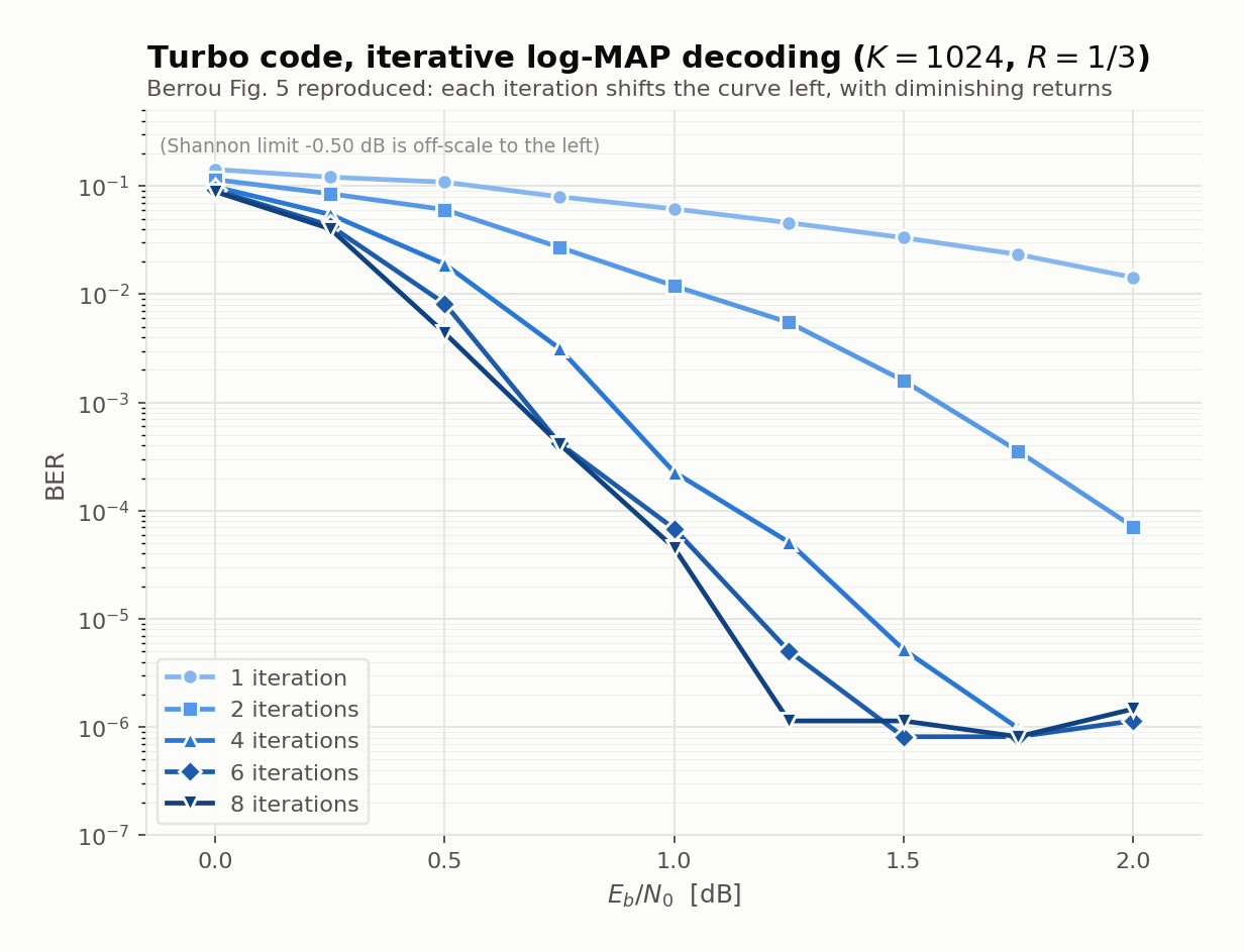

Two features of that picture are worth naming, because both recur throughout this series. The first is the diminishing returns already described: the early iterations buy whole decibels, the later ones buy almost nothing, so a sensible decoder stops early rather than running a fixed large count. The second is the flattening at the bottom right, where every curve converges onto the same floor regardless of iteration count. That floor is not a simulation artifact and no amount of extra iterating will remove it, because it is a property of the code rather than the decoder. Explaining exactly where it comes from is the business of the next entry.

The “further precautions” phrase is not idle. Berrou observed in his experiments that the BER could increase from one iteration to the next: the residual correlation we flagged above lets overconfident extrinsic values feed on themselves. His remedy is a soft saturation applied to the extrinsic quantity $z_k$ before it is passed on:

$z_k \;\leftarrow\; \frac{z_k}{1 + \theta\,|z_k|}, \qquad \theta = 0.15.$

Small values pass almost untouched; large values are compressed toward a ceiling. Modern implementations achieve the same effect by multiplying $L_e$ by a constant near 0.7, or by clipping $|L_e|$ at a maximum. Recognize this as the same medicine prescribed in the previous section for Max-Log-MAP, and the same medicine min-sum LDPC decoders take: wherever an iterative decoder’s messages run more confident than the evidence justifies, a scalar damping factor restores stability. Three superficially different tricks, one phenomenon.

For the record, here are the parameters behind the headline result, from Berrou’s own experiment:

Parameter	Value
Constituent codes	RSC, $K=5$ (memory 4), $G_1=37_8$ feedback, $G_2=21_8$ feedforward
Constituent rate	$R_1=R_2=2/3$ after puncturing
Overall rate	$R = 1/2$
Interleaver	$256\times256$ block, $N = 65536$ bits
Iterations	up to 18
Extrinsic damping	$z_k \leftarrow z_k/(1+\theta
Headline result	BER $10^{-5}$ at $E_b/N_0 = 0.7$ dB
Shannon limit at this rate	about 0.2 dB, so the gap is roughly 0.5 dB

A Numerical Example: Input-Weight Analysis

Everything so far explains how a turbo code is decoded. This last section starts to explain why it is good, by tracing an RSC encoder’s response to the simplest possible inputs. Take the small 4-state RSC(7,5): feedback polynomial $1+D+D^2$, feedforward $1+D^2$. The state is the register pair $(a_{k-1}, a_{k-2})$, the recursion is $a_k = d_k \oplus a_{k-1} \oplus a_{k-2}$, and the parity output is $p_k = a_k \oplus a_{k-2}$.

First, feed it a single 1 followed by zeros: $d = 1,0,0,0,0,\dots$ starting from state $(0,0)$.

$k$	$d_k$	$a_k$	$p_k$	next state
0	1	1	1	(1,0)
1	0	1	1	(1,1)
2	0	0	1	(0,1)
3	0	1	0	(1,0)
4	0	1	1	(1,1)
5	0	0	1	(0,1)

Watch the state column: after the impulse, the register cycles through $(1,0) \to (1,1) \to (0,1)$ with period 3 (which is $2^m - 1$ for a primitive feedback polynomial of degree $m = 2$) and never returns to $(0,0)$. The parity stream is periodic and never stops: this is the infinite impulse response promised earlier, now visible in a table. A weight-1 input drives an RSC encoder into an error event of infinite parity weight. Two immediate consequences. First, the smallest input weight that can produce a finite-weight error event in a recursive encoder is 2; in the standard notation, $w_{\min} = 2$, whereas a nonrecursive encoder has a finite impulse response and $w_{\min} = 1$. Second, you cannot terminate an RSC trellis by appending $M$ zeros the way you terminate an ordinary convolutional code: zeros at the input leave the feedback loop cycling forever, and forcing the state home requires feeding the register contents back at the input (a switched tail). This is exactly why the second constituent encoder often goes unterminated, and why its $\beta$ recursion gets the uniform initialization mentioned in the derivation.

Now feed it a weight-2 input with the two 1s separated by the cycle period: $d = 1,0,0,1,0,0,\dots$

$k$	$d_k$	$a_k$	$p_k$	next state
0	1	1	1	(1,0)
1	0	1	1	(1,1)
2	0	0	1	(0,1)
3	1	0	1	(0,0)

The second 1, arriving exactly one period after the first, cancels the circulating pattern and closes the loop back to the zero state. Input weight $w = 2$, parity weight $z = 4$, constituent codeword weight 6. This is the shortest finite-weight error event the encoder has.

Now assemble the consequence for the concatenated code. Build the rate-1/3 PCCC from two copies of this RSC(7,5). The dominant low-weight event comes from a weight-2 input that closes the loop in both encoders (both the original pattern and its interleaved image hitting a period-multiple spacing), and its total transmitted weight is

$d_{\text{eff}} = \underbrace{2}_{\text{systematic}} + \underbrace{4}_{\text{parity 1}} + \underbrace{4}_{\text{parity 2}} = 10.$

This quantity, the minimum total weight over weight-2 inputs, is called the effective free distance. Compare it with the constituent code’s own free distance: $d_{\text{free}} = 5$, achieved by the weight-3 input $d = 1,1,1$, which produces parity $1,0,1$ for a total of $3 + 2 = 5$ (trace it through the recursion yourself; it is a three-row table). Here is the counterintuitive design lesson hiding in that comparison: when you choose constituent codes for a turbo code, $d_{\text{free}}$ is not the figure of merit. You optimize $d_{\text{eff}}$, the distance associated specifically with weight-2 inputs, because weight-2 events turn out to be the only ones that survive the interleaver’s protection in quantity. Fifty years of coding theory had taught designers to maximize minimum distance above all else; turbo codes quietly demote it. Justifying that demotion (why weight 2 and only weight 2, and what exactly the interleaver does to the rest) requires the analysis machinery of the next page.

Check Yourself

Before moving on, test the machinery. Answers are folded below.

1. The second RSC encoder produces a systematic output too. Why is it never transmitted?
2. Why does the iterative decoder require MAP (BCJR) constituent decoders rather than the cheaper and more familiar Viterbi algorithm?
3. Why must the decoders exchange only the extrinsic term $L_e$, rather than the full posterior $L(d_k)$? What goes wrong otherwise, and what is the observable symptom?
4. Why can’t you terminate an RSC trellis by appending $M$ zero bits, as you would for an ordinary convolutional encoder?
5. Your freshly written turbo decoder improves for three iterations and then degrades. Name two likely causes and their fixes.
6. A constituent RSC code has $d_{\text{free}} = 7$, achieved by a weight-3 input, while its weight-2 inputs produce minimum parity weight 6. What is $d_{\text{eff}}$ of the rate-1/3 PCCC built from two copies, and why is the $d_{\text{free}} = 7$ figure a distractor?

Answers

1. It is a permutation of the systematic bits already transmitted alongside encoder 1’s parity: zero new information at the receiver, pure rate loss. The de-interleaver at the decoder recovers the ordering for free.

2. Viterbi outputs the most likely sequence as hard bits. The iterative loop needs, for each individual bit, a soft reliability (an LLR) that the other decoder can use as a prior, and it needs the a posteriori probability per symbol, which is exactly what BCJR computes with its forward-backward sweeps.

3. The posterior $L(d_k)$ contains the a priori term $L_a$ that the other decoder itself supplied, plus the channel term $L_c y^s_k$ that both decoders already see. Passing it whole returns the other decoder’s own opinion to it disguised as fresh evidence, creating positive feedback: the loop converges confidently to whatever it believed first. The proved decomposition $L = L_c y^s + L_a + L_e$ shows that only $L_e$, built from the parity observations of the other bits, is genuinely new. The classic symptom of passing the full posterior is a BER that improves for two or three iterations and then worsens.

4. Because the shift register stores the fed-back sequence $a_k$, not the input $d_k$. With zeros at the input, the recursion $a_k = 0 \oplus a_{k-1} \oplus a_{k-2}$ keeps the register cycling through its period-$(2^m-1)$ orbit indefinitely, as the weight-1 table shows. Forcing the encoder home requires feeding the register contents back into the input (a switched tail); if you skip termination, the $\beta$ recursion must start from a uniform distribution over states, a small real loss.

5. (a) Passing the full APP instead of the extrinsic term: fix by subtracting $L_c y^s_k$ and $L_a$ before the exchange. (b) Overconfident extrinsic values with no damping, especially under Max-Log-MAP, which systematically overestimates reliability: fix with Berrou’s $z/(1+\theta|z|)$ saturation at $\theta = 0.15$, or scale $L_e$ by roughly 0.7. A third candidate worth checking: a mismatch between the interleaver and de-interleaver index maps.

6. $d_{\text{eff}} = 2 + 6 + 6 = 14$: systematic weight 2 plus minimum weight-2 parity from each encoder. The free distance is a distractor because it is achieved by a weight-3 input, and the next page shows that the interleaver suppresses weight-3 events far more strongly than weight-2 events; only the weight-2 events survive in quantity, so their distance is the one that governs performance.

Where This Leaves Us

Berrou, Glavieux and Thitimajshima built a code of length 196,608 that no decoder ever confronts whole: two weak recursive systematic convolutional encoders, coupled through a 65,536-bit interleaver, decoded by two BCJR modules passing carefully filtered opinions back and forth. We derived the full decoder on this page: the forward-backward recursions from the Markov property of the trellis, the branch metric from the Gaussian channel, and, rather than asserting it, we proved the three-term decomposition $L = L_c y^s + L_a + L_e$ that identifies exactly which part of a decoder’s belief is safe to share. Two ingredients carried all the weight, and neither is obvious: the constituent encoders must be recursive, and the decoders must exchange only extrinsic information, a principle that already lived, unnoticed, in Gallager’s 1963 update rule. Around the edges we collected the practical folklore: Max-Log-MAP’s overconfidence and its 0.7 scaling factor (the same disease and cure as min-sum LDPC decoding), Berrou’s damping fix, the impossibility of terminating an RSC with zeros, and the strange arithmetic of the worked example, where the code’s real vulnerability is weight-2 inputs and the design target is $d_{\text{eff}}$, not $d_{\text{free}}$.

But notice what this page has not done. It showed that the construction works, at 0.7 dB, to five nines of the field’s astonishment; it traced how every box in the decoder computes; and it gestured, through one worked example, at why recursion matters. The actual explanation is still owed. Why exactly does the interleaver reward $w_{\min} = 2$ and punish nothing else? Why does an encoder property (recursion) matter when the recursive and nonrecursive encoders generate the same code? And why does performance improve with interleaver length in the coefficient but never in the slope? Berrou’s paper contains almost no theory; it took Benedetto and Montorsi three more years to supply it. That analysis, the uniform interleaver and the interleaver-gain exponent $N^{1-w_{\min}}$, is the next page.