What an Embedded System Is, and How It's Designed

Most computers in the world aren’t the one you’re reading this on. They’re wedged inside a car’s brake controller, a pacemaker, a coffee machine, a factory robot arm: devices that are computers on the inside but don’t advertise it, because being a general-purpose computer was never the point. This is the first of a set of notes working through two textbooks on how those systems actually get designed: Wolf’s Computers as Components and Lee and Seshia’s Introduction to Embedded Systems (I’ll shorten that to “LS” from here on, the way the book itself does). This phase covers the ground both books lay before getting technical: what actually separates “embedded” from “general-purpose,” and the design process both books build their later chapters around.

What Counts as “Embedded,” and Why Microprocessors Won

An embedded computer system is any device with a programmable computer inside it that isn’t itself meant to be a general-purpose computer: a fax machine, not a PC, even though a PC is very likely what you’d use to build the fax machine’s firmware. That distinction sounds almost too simple to matter, but it explains a piece of history that’s easy to miss: the very first microprocessor, Intel’s 4004 in 1971, wasn’t built for general computing at all. It was designed for a calculator. Embedded computing isn’t a niche market that microprocessors eventually spread into; it’s where microprocessors started.

That accident of history is also why microprocessors beat custom logic, and it’s worth sitting with the reasoning rather than taking it as given. Fetching and decoding an instruction is, in a real sense, wasted work compared to a custom circuit that just does the thing, with no instruction stream to interpret at all. And yet programmable chips won almost everywhere. Three reasons: CPU vendors pour far more R&D into raw speed and process technology than a small custom-logic team could ever match; a single programmable chip reused across many products is often smaller, in total gate count, than N custom blocks that each sit idle most of the time; and (probably the most important one long-term) programmability decouples the hardware and software design tracks, so a company can ship a whole family of products by changing firmware instead of taping out a new chip for every variant.

There’s a deeper idea underneath all of this that the book calls the “physics of software”: software isn’t abstract. It’s electrons moving through a real circuit, so every instruction costs real time and real energy. That’s why performance and power analysis show up as first-class engineering topics in embedded design, rather than something you profile at the end if there’s time left over.

It’s also why embedded design is harder than writing software for a PC, in ways that aren’t just “more constrained.” A late-but-correct answer is a bug: deadlines are part of correctness, not a performance nice-to-have. A single device often has to satisfy several real-time rates simultaneously (audio and video in a media stream have different deadlines, and both must be met). Budgets for cost and power are tight, teams and schedules are small, and (this one is easy to underestimate) the debugging environment itself is worse: no keyboard, no screen, limited visibility into what the device is actually doing, cross-compiled toolchains talking to hardware over a wire.

One more framing from Wolf’s opening chapter is worth keeping in mind for the rest of this series, because it previews the shape the material takes later: real-time performance has to be reasoned about across nested layers, from the CPU itself, then the platform (buses, I/O), then a single program, then a task inside a multitasking system, then a whole multiprocessor. Each layer’s behavior is shaped entirely by the layer underneath it. That’s basically a table of contents for an embedded systems course, and it’s roughly the order this notes series will drift toward as well.

The Design Process: Top-Down, Then Corrected Bottom-Up

Wolf lays out a design process that looks deceptively linear on a first pass: requirements → specification → architecture → components → system integration. Read it that way and you’ll miss the more useful part, which is the second half of the sentence: refined top-down, but corrected bottom-up when your early estimates turn out to be wrong, which they usually are, since early decisions have to rely on guesses about things you don’t actually know yet, like how fast, how much memory, how much bus bandwidth you’ll need.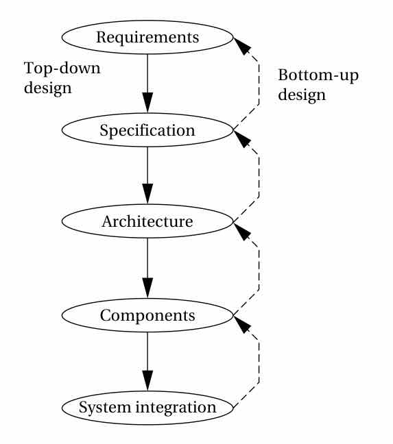

At every one of those steps, you’re tracking the same three goals (manufacturing cost, performance, power) and performing the same three tasks: analyze (can we still meet spec?), refine (add detail), verify (did we just break something we already met?). Two of those stages deserve to be pulled apart even though it’s tempting to merge them. Requirements are the informal customer wishlist: functional needs plus nonfunctional ones like performance, cost, size, and power. The specification is different in kind, not just in detail: it’s a precise contract between customer and architect, unambiguous enough that you could actually build from it. Skipping straight from a wishlist to building is the classic novice mistake, and it’s expensive precisely because you only discover your wrong assumptions once the system already exists.

Architecture answers how, not just what: it’s a structural description, typically a block diagram, and good practice is to draw one abstract, implementation-agnostic system-level diagram first, and only then split it into separate hardware and software block diagrams. That ordering matters: it keeps early architectural decisions from getting quietly biased by whatever happens to be easy in one particular implementation. Components themselves are usually a mix of off-the-shelf parts (a CPU, memory chips, a GPS receiver module) and custom-built ones (a PCB layout, application code); you reuse wherever you can, because standard parts are both cheaper and better optimized than what a small team could build from scratch. And system integration is where bugs surface, which is exactly the phase embedded systems are worst-equipped to debug, thanks to that same poor observability, so the discipline is to plan test points and incremental bring-up back in the earlier phases, not scramble for them once everything’s already assembled.

A Shared Language for Structure and Behavior: UML

Both books lean on UML to make specifications precise enough to build from, and it’s worth knowing the vocabulary now, because it resurfaces in a more formal shape once these notes get into state-machine modeling in the next phase. On the structural side: an object is an instance with state (its attributes), and a class is the type that defines those attributes plus the operations you’re allowed to touch them through. That restriction, that you can only reach an object’s state via its declared operations, is exactly what lets an implementation change later without breaking whatever’s calling it. Objects relate to each other in a few standard ways: association (they communicate, with no ownership implied), aggregation (whole/part), composition (aggregation where the whole also hides its parts from outside view), and generalization (inheritance, including the multiple kind).

On the behavioral side, UML gives you state machines: states plus transitions triggered by events, where an event can be a signal (asynchronous), a call event (behaves like a procedure call), or a time-out (fires after some duration); and sequence diagrams, which read top-to-bottom in time and show the order messages pass between several objects’ “lifelines.” Sequence diagrams are good at nailing down one concrete scenario; they’re the wrong tool if you’re trying to show every possible branch at once.

A Worked Example: The Model-Train Controller

Wolf walks the entire requirements → conceptual-spec → detailed-spec pipeline on a system small enough to hold in your head: a model-train controller. The big lesson isn’t really about trains. It’s this: build on an existing standard (in this case DCC, the digital command control protocol model railroaders already use) rather than inventing your own from scratch. Doing that buys you two things at once: it cuts the amount of work you have to do, and it buys interoperability with everyone else’s hardware for free. There’s a companion warning worth keeping, too: “overstandardization.” Only standardize the parts that genuinely need to interoperate; padding a standard out with things that don’t need to be shared just makes it heavier and less attractive to adopt.

DCC’s packet format is specified as a compact regular expression, and it’s a nice small example of using formal notation to pin down a bit-level protocol without any ambiguity:

$$P\ S\ A\ (s\ D)^{+}\ E$$

where $P$ is the preamble (at least ten 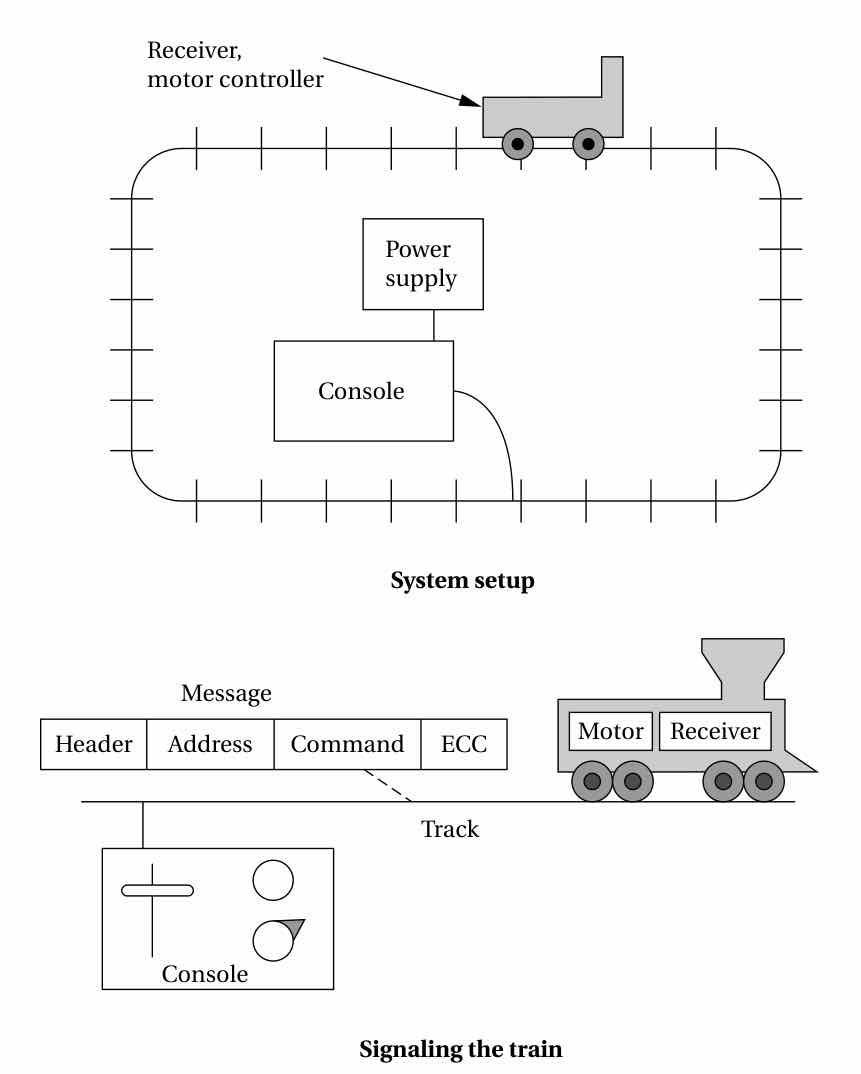1 bits), $S$ is the packet start bit (0), $A$ is the address byte, $s$ is a data-byte start bit, $D$ is a data byte, and $E$ is the end bit. The $(s\ D)^{+}$ means “one or more (start-bit, data-byte) pairs”: plain regular-expression syntax, doing real engineering work.

There’s a meta-lesson buried in this exercise, too, and it generalizes well beyond model trains: writing the specification teaches you things about the system you’re specifying. Deciding to spend 3 bits on a message-type field, for instance, forces the concrete, implementation-relevant realization that you’ve just bought yourself 5 spare codes for whatever gets added later. You don’t find decisions like that by thinking about the system in the abstract; you find them by trying to pin it down precisely enough to build.

Cyber-Physical Systems: Where Computation Meets Physics

Lee and Seshia frame the whole subject differently, and it’s worth holding both framings side by side. A cyber-physical system (CPS) is computation integrated with a physical process, where the system’s actual behavior is defined by both halves together: CPS lives at the intersection of cyber and physical, not their union. You can’t fully understand the computation and the physics separately and then just glue the two understandings together at the end; the interesting behavior only shows up once they’re coupled.

The motivating examples LS reaches for all share the same shape: beating-heart surgery robots, cooperative-traffic intersections, fly-by-wire aircraft with flight envelope protection and soft walls. In every one of them, computation sits between a human’s intent and the physical actuation that follows from it, trusted to keep the whole system safe. Structurally, a CPS is a physical plant plus one or more platforms (sensors, actuators, one or more computers, an OS) connected by a network fabric. A feedback control loop is what you get when a platform’s computation reads its own sensor and drives its own actuator, guided by a control law.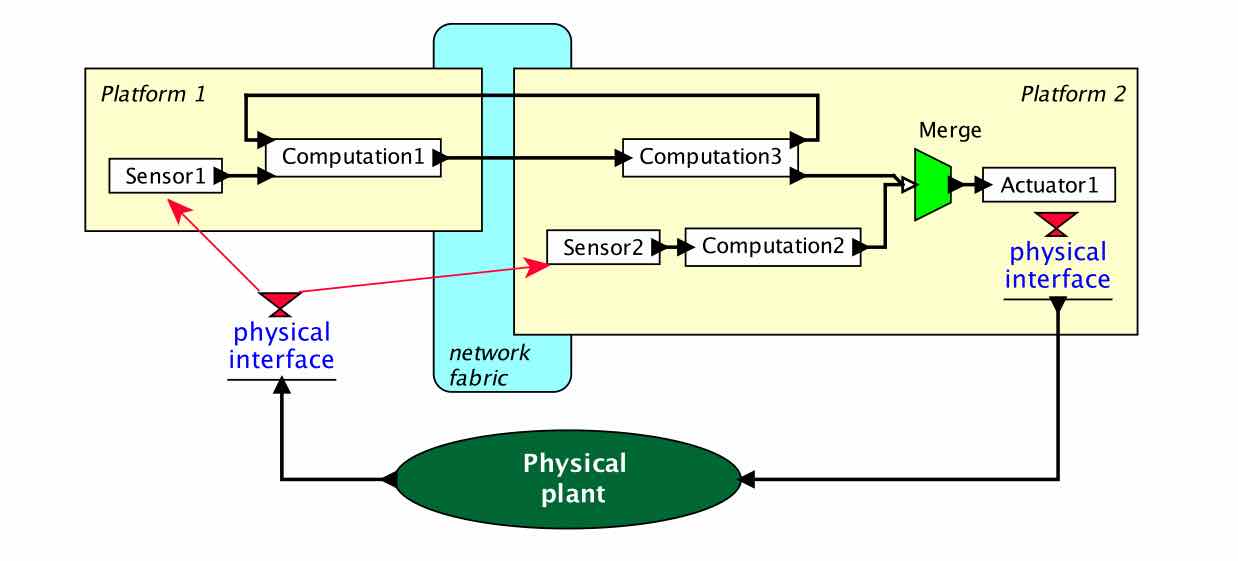

LS’s running example throughout the book is a quadrotor called STARMAC, and it’s worth noticing why it’s such a good teaching example: it needs control algorithms (which in turn need both continuous dynamics and discrete state machines for flight modes like takeoff, hover, and land), it has real weight and energy trade-offs, and it needs to operate autonomously, which drags in localization and fault handling. Almost every later chapter in the book maps onto some piece of this one machine.

That leads to LS’s version of the design process, which reframes Wolf’s five stages as three intellectual activities, iterating rather than running in a straight line: Modeling asks what a system does, understanding by imitation. Design asks how, structured creation of artifacts. Analysis asks why it does, or doesn’t, do what the model claims, understanding by dissection.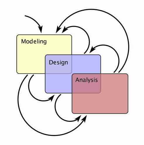

A model, in this framing, is itself a system. It has fidelity (how accurately it reflects the real thing), and it necessarily abstracts, meaning it leaves things out on purpose. The discipline is never confusing the model with the thing it models. There’s a line from this chapter worth remembering on its own, because it’s the cleanest argument for why specification matters that I’ve come across: “A design without [a specification] cannot be right or wrong, it can only be surprising.”

Two Vocabularies, One Loop

Wolf and Lee-and-Seshia describe the same underlying process, just from different angles. Wolf’s version (requirements → specification → architecture → components → integration) is the engineering/product view, with concrete deliverables like charts and UML diagrams at each stage. LS’s version (modeling → design → analysis) describes the same loop as three intellectual activities rather than five process stages. Line them up and the mapping is fairly clean: Wolf’s “specification” step is roughly LS’s “modeling” step, and Wolf’s “verify” task at each stage is roughly LS’s “analysis.” It’s worth keeping both vocabularies active, since later phases will reach for whichever book’s version fits the topic better.

The thread to carry forward: an embedded system is a programmable computer built into a product rather than sold as one, and that one constraint (real-time deadlines, tight cost and power budgets, small teams, and a debugging environment with poor visibility) is what makes designing one a genuinely different discipline from writing software for a general-purpose machine. The next phase gets concrete about what “system behavior” formally means: continuous dynamics, discrete state machines, and the hybrid combination of the two that’s the actual mathematical shape of most cyber-physical systems.