Modeling Foundations: Dynamics, State Machines, Concurrency

Phase 0 ended with a promise: continuous dynamics, discrete state machines, and the hybrid combination that’s the real mathematical shape of most cyber-physical systems. This phase makes good on it. It works through five chapters of Lee and Seshia in sequence: continuous dynamics, discrete dynamics, hybrid systems, composing state machines together, and finally the general question of what “concurrent computation” even means. Each one builds directly on the last, so it’s worth reading in order even though the section headings below make it look like five separate topics.

Continuous Dynamics: The Physical Half

A continuous-time signal is just a function $f:\mathbb{R}\to\mathbb{R}$ from time to value, and it’s the natural way to describe something like the position or orientation of a physical object moving through space. A rigid body’s full pose needs six degrees of freedom: three for position, three for orientation (roll, pitch, yaw), shown below for a helicopter, which is the example LS carries through this entire chapter.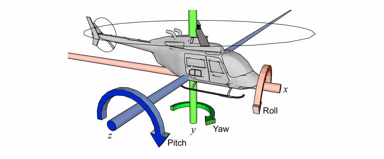

The physics underneath is Newton’s second law, $\mathbf{F}=M\ddot{\mathbf{x}}$, which generalizes to rotation via torque, $\mathbf{T}=\mathbf{I}(t)\ddot{\boldsymbol\theta}(t)$, where $\mathbf{I}(t)$ (the moment of inertia) is a full 3×3 matrix that depends on the body’s geometry and orientation, and only collapses to a single scalar for symmetric bodies like a sphere. In practice you almost never need the full six-dimensional picture. Model-order reduction is the deliberate move of dropping the dimensions that don’t matter for the question you’re actually asking: a helicopter’s yaw-stabilization problem, for instance, only needs the relationship between torque and angular velocity around one axis, not the full six-degree-of-freedom position-and-orientation picture. Throwing away realism on purpose, to end up with a model you can actually reason about, is the point, not a shortcut you’re settling for.

LS builds up a small, reusable visual vocabulary for this kind of system: an actor is a box $S: X \to Y$ mapping an input signal (or several) to an output signal, and actors compose by wiring an output into an input; this is literally the diagram language Simulink and LabVIEW are built on. A few actors recur constantly: Scale ($y = ax$), Integrator (its output is the running integral of its input, plus an initial value), and Adder (sums, or subtracts, several inputs).

Once you have actors, you can ask precise questions about them instead of vague ones, and each of these has an exact definition worth holding onto rather than approximating from intuition:

• Causal: the output up to time $\tau$ depends only on the input up to time $\tau$. Strictly causal tightens this to exclude the present instant: output at $\tau$ depends only on input strictly before $\tau$. This matters for feedback: a loop needs at least one strictly-causal actor somewhere in the cycle, or it ends up referring to itself at the same instant and is simply ill-defined.
• Memoryless: output at $t$ depends only on input at $t$ (an Adder is memoryless; an Integrator very much isn’t).
• Linear: satisfies superposition, $S(a x_1 + b x_2) = aS(x_1)+bS(x_2)$.
• Time-invariant: commutes with a delay actor; shift the input in time, and the output shifts by exactly the same amount.
• LTI (linear + time-invariant) is the sweet spot where analysis stays tractable, and it’s usually worth approximating a system as LTI whenever that’s a reasonable stretch.
• BIBO stable: every bounded input produces a bounded output.

The helicopter tail-rotor example is where these definitions earn their keep. A bare integrator model with no feedback is BIBO unstable: feed it a constant, perfectly bounded torque, and the angular velocity grows without bound forever. Add proportional feedback control instead (an error signal $e = \psi - \dot\theta_y$ driving a control torque $T_y = K\cdot e$), and the closed loop becomes exponentially stable for $K>0$:

$$\dot\theta_y(t) = \dot\theta_y(0)\, e^{-Kt/I_{yy}}$$

and unstable for $K<0$. This is the single clearest illustration of a cyber-physical system in the whole chapter: a plain software gain constant, $K$, literally determines whether a physical helicopter is stable or not.

Discrete Dynamics: State Machines

Continuous components evolve smoothly and get modeled with ODEs, as above; discrete components evolve through abrupt, instantaneous reactions, and the natural tool for those is a state machine instead. A pure signal carries no value at all, only presence or absence at each instant (the discrete-time analog of a continuous-time signal), though a signal can also carry a value when present, the way a garage counter’s count output does. A discrete signal, more precisely, is one whose present-times can be put in order-preserving correspondence with the natural numbers: you can count off its events in order. One catch worth flagging: discreteness isn’t compositional. Merging two discrete signals can produce a signal that isn’t discrete anymore.

State is best understood as a summary of everything about the past that matters for future behavior: an Integrator’s state is its accumulated area so far; a Counter’s state is its running count. A finite-state machine (FSM) is simply a state machine with finitely many states: bubbles for states, curved arrows for transitions, each labeled guard / action, where a guard is a boolean predicate on inputs (or, in extended machines, variables) and an action assigns output values. Anything not mentioned in an action is implicitly absent. If no guard fires and every input is absent, the machine stutters (no state change, no output), which is subtly different from an explicit self-loop. A dashed default transition (true /) makes that “otherwise do nothing” case visible on the diagram; it’s convenience notation, always reducible to an ordinary transition with the negated guard.

Formally, an FSM is a 5-tuple $(States, Inputs, Outputs, update, initialState)$ with

$$(s_{i+1}, y_i) = update(s_i, x_i)$$

where the next state and this reaction’s output are both a function of the current state and current input. This precise form is what later chapters’ proofs, on composition and verification, actually build on once diagrams get too large to draw by hand.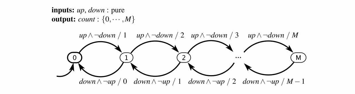

A few distinctions are easy to blur together but worth keeping separate. Mealy machines (which this book uses throughout) produce output on the transition, so output can depend on the current input; Moore machines produce output from the current state alone, which makes them always strictly causal. Mealy machines tend to need fewer states, and the two forms are interconvertible. Determinism (at most one transition enabled per state/input pair) is a structural property about the guards; determinacy (always producing the same output for the same input) is a semantic one. Every deterministic machine is determinate, but not the other way around. Receptive means at least one transition is always enabled, so the machine never gets stuck; the implicit default transition in the graphical notation guarantees this automatically. Put determinism and receptiveness together and you get exactly one transition per input, always.

Real machines usually need more state than you’d want to draw as individual bubbles. Extended state machines solve this by adding ordinary variables, read and written on transitions, so a counter up to some large $M$ needs a handful of bubbles instead of $M$ of them. The transition syntax grows to guard / output-action set-action(s), and set-actions are evaluated after the guard and output, using the pre-update variable values. With $n$ bubbles and $m$ variables each ranging over $p$ values, the state space is bounded by

$$|States| = n \cdot p^{m}$$

This is an upper bound, since not all of that space is necessarily reachable.

The thermostat is the standard example for hysteresis: using two thresholds instead of one (heat comes on below 18°, goes off above 22°, straddling a 20° setpoint) prevents chattering: rapid on/off switching right at the threshold. It’s a specific, useful kind of memory with a nice property called time-scale invariance: stretch or compress the input signal in time, and the output response stretches or compresses by exactly the same factor.

Finally, nondeterminism: a machine is nondeterministic if some state/input pair enables more than one transition. This is useful in two quite different ways. It can model an environment you don’t want to pin down exactly: “a pedestrian might or might not arrive,” without modeling actual foot traffic. Or it can express deliberate underspecification in a requirement: “lights must cycle red → green → yellow,” while leaving exact timing unconstrained. Nondeterminism is not probability: a nondeterministic model makes no claim about likelihood, only about the set of behaviors that are possible; a stochastic model is the genuinely distinct, probability-bearing version of the same idea. Formally, the update function becomes a relation, $(s_{i+1}, y_i) \in possibleUpdates(s_i, x_i)$, and a single initial state becomes a set of initial states. A behavior is one consistent assignment of inputs and outputs across all reactions; for a nondeterministic machine, one input sequence can admit several valid behaviors, and the set of all of them is the machine’s language. A computation tree enumerates every possible trace, branching at each nondeterministic choice, which is useful for visualizing that some “bad” behavior is unreachable, and a direct preview of the model-checking material later in the book.

Hybrid Systems: Where the Two Meet

This is arguably the single most important modeling idea in the whole book for cyber-physical systems, because it’s the literal mathematical object where “cyber” (modes, discrete logic) and “physical” (continuous dynamics) actually meet: attach a continuous, time-based system to every state of an FSM. A modal model is an FSM where each state (now called a mode, to avoid confusing it with the mode’s own internal state) has an associated refinement: a continuous system describing the dynamics of outputs and continuous variables while the machine is in that mode. It’s worth being careful with the terminology here, because a hybrid system genuinely has two kinds of state at once: discrete state (which mode you’re in) and continuous state (the refinement’s internal variables, such as a clock, a position, whatever it’s tracking).

Continuous inputs generalize the plain FSM picture in one important way: a transition now fires the instant its guard becomes true, not just “at the next reaction,” and inputs and outputs no longer have to be absent between reactions. That’s what lets a discrete FSM coexist with a shared, continuous timeline.

The simplest nontrivial hybrid systems are timed automata (Alur and Dill, 1994), where every mode’s refinement is nothing more than a clock, $\dot s(t) = a$ for some constant rate $a$ (usually $a=1$, an ordinary stopwatch). Despite that simplicity, clocks plus guards plus reset actions (s := 0) are enough to build minimum-dwell-time behavior (“the heater must stay on for at least $T_h$ seconds”), which is a cheap alternative to hysteresis for preventing chattering, at the cost of losing hysteresis’s nice “settles near the setpoint” property.

Refinements aren’t limited to clocks, though. The sticky-masses example uses a full ODE per mode, one per Newton’s-law spring system, and the interesting part is what happens at a mode transition: it can carry a set-action that reinitializes the continuous state. On collision, for instance, momentum conservation sets the new combined-mass velocity,

$$\dot y(t) = \frac{m_1 \dot y_1(t) + m_2 \dot y_2(t)}{m_1 + m_2}$$

and the “together” mode’s ODE picks up from there. That’s the general pattern for modeling any abrupt physical event: a collision, a mode switch, a saturation limit.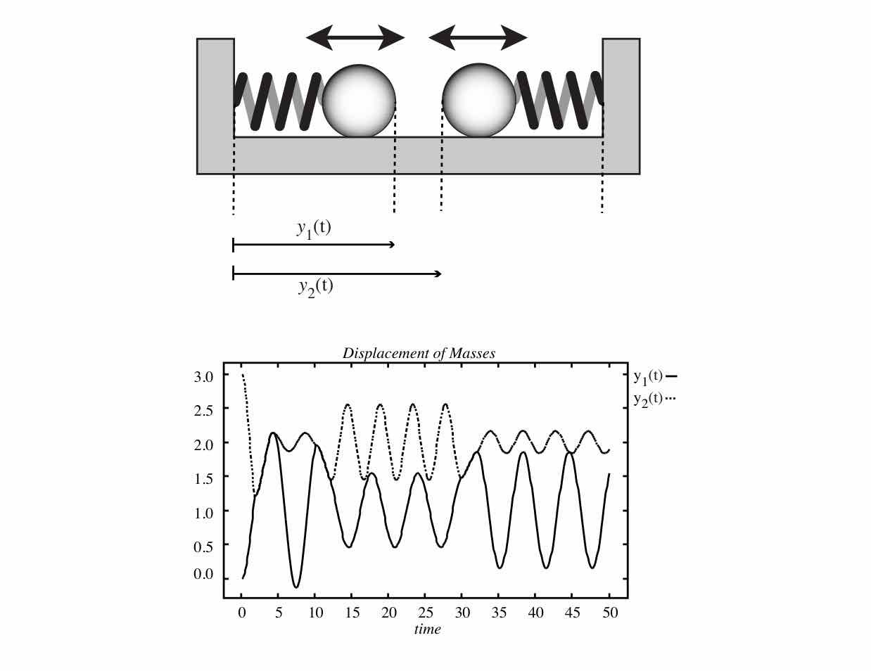

There’s a genuine pathology worth watching for once you start building your own hybrid models: a Zeno system takes infinitely many discrete transitions in a finite time interval, at least in the idealized math. The classic case is a bouncing ball with inelastic bounces (energy-loss factor $a<1$): free-fall refinement $\ddot y(t) = -g$, with each bounce resetting the velocity via $\dot y(t_1) := -a\,\dot y(t_1^-)$. Each bounce-to-bounce interval shrinks geometrically, so the model predicts infinitely many bounces before some finite time, which obviously doesn’t happen to a real ball, since it eventually just stops. Zeno behavior is a red flag pointing at your model, not the physical system.

Control systems in this framing decompose into a plant (the physical process), an environment, sensors, and a two-level controller: a supervisory controller that’s discrete and picks which mode or strategy is active, sitting on top of a low-level controller that’s continuous and picks the actual control inputs within whichever mode is active. That’s exactly the hybrid-system structure again: the supervisory logic is the mode graph, and the low-level control is each mode’s refinement. LS’s AGV (warehouse robot) example ties the whole chapter together this way: a photodiode array estimates lateral error $e(t)$ off a painted line, and supervisory control picks among four modes (stop, straight, left, right) based on two thresholds $\epsilon_1 < \epsilon_2$ on $|e(t)|$, while each mode’s low-level refinement is a simple constant-turn-rate ODE. It’s a template worth remembering for any “keep some measured error small” control problem, not just line-following robots.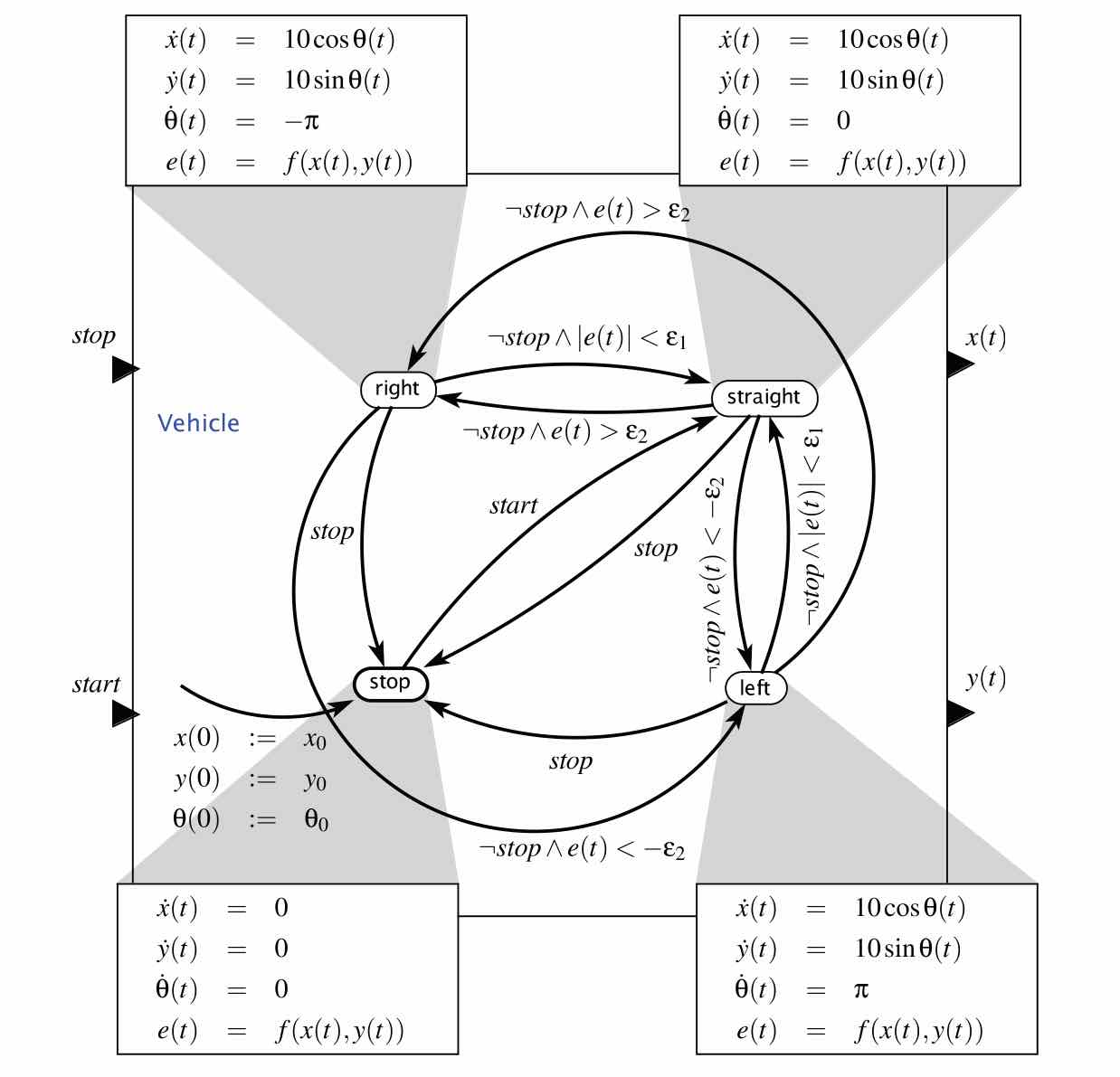

Composing State Machines

Large systems obviously can’t be one giant hand-drawn bubble diagram, so the natural next question is how smaller state machines combine into bigger ones; the chapter’s real lesson is that “composition” isn’t one thing. The same visual syntax, boxes and wires, can carry several genuinely different semantics, and being precise about which one you mean is itself a skill worth developing deliberately.

Side-by-side composition takes two machines with disjoint inputs, outputs, and variables and combines them into one actor. If they react synchronously (both simultaneously, every reaction), the composite is nicely modular: from outside, it looks like a single atomic FSM, and determinism is compositional here, meaning two deterministic machines composed synchronously always yield a deterministic composite. You can always write the composite as one FSM whose state space is the cross product of the two components’ state spaces:

$$States_C = States_A \times States_B$$

though not every state in that cross product is necessarily reachable. If instead the machines react asynchronously (independently), “independently” turns out to have at least four distinct readings worth telling apart: exactly one machine reacts each step, chosen nondeterministically; either or both may react; or the same two options, except an external scheduler makes the choice instead of nondeterminism. Interleaving semantics has a real, not just theoretical, hazard: an input event meant for machine A can simply get dropped if the nondeterministic choice happens to pick machine B that step. And asynchronous composition doesn’t preserve determinism the way the synchronous case does: composing two deterministic machines asynchronously generally yields a nondeterministic composite. Once you add shared variables on top of asynchrony, atomicity itself becomes an open question: does a write happen “before” a same-reaction read? This is precisely the state-machine-diagram version of the race conditions that resurface later with real threads and interrupts.

Cascade composition feeds one machine’s output into another’s input, and has to type-check: A’s output type must fit inside whatever B’s input port accepts. A synchronous cascade reacts as “simultaneous and instantaneous,” even though A’s output causally affects B within the very same step, and a full reachability analysis on the composite can reveal that some naively-expected intermediate state is actually never reached at all; composing a traffic light with a pedestrian light, for instance, can prove the unsafe “both green” state unreachable by construction. General composition allows arbitrary interconnection of side-by-side and cascade pieces, which can create feedback cycles (A’s output feeds B, and B’s output feeds back into A), and that raises a question neither side-by-side nor cascade composition alone can answer: which machine reacts first? This chapter deliberately leaves the question open; it’s resolved by the synchronous-reactive model of computation, coming up next.

Machines can also nest. In a hierarchical state machine (Statecharts-style), a state can have its own refinement (a nested FSM), so “being in state B” really means “being in one of B’s sub-states.” Reaction order is depth-first: the deepest active refinement reacts first, then its container, working outward. If an inner and an outer transition are both enabled in the same reaction, both actions execute in sequence, with the later one winning on any conflicting write, but the machine ends up exactly where the outer transition says; it never visibly passes through the inner target state. A hollow-arrowhead reset transition always resets a refinement to its own initial substate on entry, regardless of history; a solid-arrowhead history transition resumes wherever the refinement was last left off, which means the composite’s effective state space is larger than the diagram alone suggests. A red-circle preemptive transition checks its guard before the refinement even gets a chance to react: if true, the refinement is skipped entirely that reaction, which is the clean way to sidestep the “which actions actually ran” ambiguity from the ordinary depth-first case.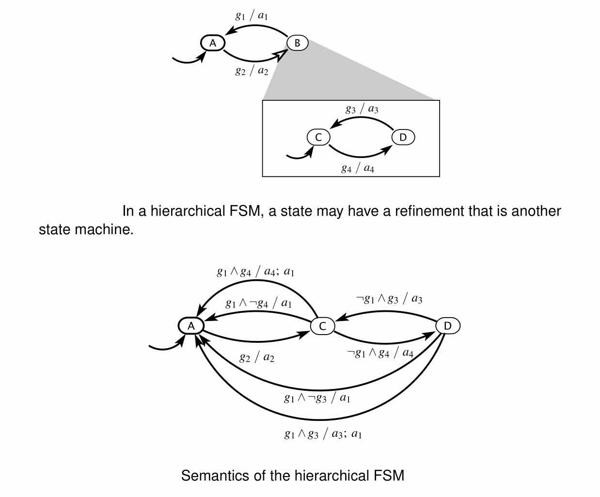

Concurrent Models of Computation

A model of computation (MoC) is really three sets of rules bundled together: what a component is, how concurrency works, and how components communicate. The previous section fixed the components as FSMs but left concurrency and communication as an open question with many valid answers; this chapter is the survey of coherent answers, and there’s a useful unifying fact underneath the whole survey: any actor network reduces to a feedback system. Side-by-side compose everything into one giant actor, and every connection that crosses back to an earlier actor becomes a self-feedback loop. That’s why the “who reacts first” conundrum from the previous section isn’t a corner case at all: it’s the general problem every model of computation in this chapter ultimately has to solve.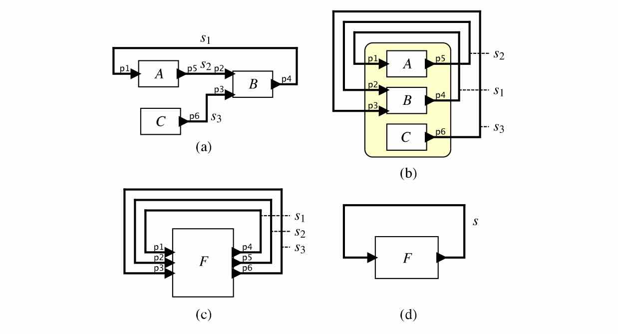

If the actors involved are determinate, the whole network is a system of equations, and its behavior at each global reaction is a fixed point of the composed function $F$:

$$s = F(s)$$

Whether that fixed point exists, whether it’s unique, and whether it can be found efficiently, are the questions that separate one model of computation from another.

Synchronous-Reactive (SR) is the strictest answer: every actor reacts simultaneously and instantaneously at each tick of a global clock, and feedback is resolved by finding a fixed point of the composed firing function at every tick. A model is well formed if every reachable state has exactly one fixed point: zero means no valid behavior exists, and more than one is treated deliberately as a modeling error rather than newly-introduced nondeterminism, specifically to preserve the property from the previous section that composing deterministic machines synchronously stays deterministic. A model is constructive if a simple must/may propagation procedure (repeatedly figuring out what output values are already forced, without exhaustive search) is enough to find that fixed point; most practical SR tools simply reject non-constructive models rather than pay for exhaustive search. This isn’t just textbook math: it’s the formal semantics behind real synchronous languages like Lustre, Esterel, Signal, and SCADE, which is what Airbus flight-control software is actually built on.

Dataflow is a much looser style of coordination: actors fire purely based on data availability (a firing rule specifying how many tokens each input needs), with no shared clock at all. Synchronous dataflow (SDF) requires each actor to consume and produce a fixed token count per firing, and that constraint buys you decidability: a linear balance equation per connection,

$$q_A \cdot M = q_B \cdot N$$

determines the firing-count ratio that guarantees bounded buffers and no deadlock. This is genuinely decidable, unlike the general dataflow case. A model with only the trivial all-zero solution is inconsistent: it can’t run forever with bounded memory. Dynamic dataflow (DDF) loosens this further, letting actors have multiple or varying firing rules (Switch/Select, the dataflow analog of goto), which is strictly more expressive but makes the bounded-buffer and deadlock questions undecidable: a direct expressiveness-for-analyzability trade. Structured dataflow recovers analyzability by nesting control explicitly (a Conditional higher-order actor wrapping sub-models) instead of routing tokens dynamically: the dataflow analog of replacing goto with structured if/for/while. And Kahn Process Networks go further still, turning actors into full concurrent processes using blocking reads and nonblocking writes on ports; Kahn’s remarkable result is that this specific discipline guarantees a determinate network (the token sequence on every connection is schedule-independent) despite unconstrained concurrent execution underneath. (A rendezvous variant, with blocking writes too, is what CSP, CCS, and Occam are built on.)

For cyber-physical systems, actual physical time often matters, not just event order, which motivates a third family. Time-triggered models keep the global clock but let computations take logical execution time between ticks (a tick-$n$ computation’s outputs aren’t visible until tick $n{+}1$), which sidesteps feedback and race issues entirely, at the cost of coarser granularity (this is what Simulink’s Real-Time Workshop does, and what underlies FlexRay in automotive systems). Discrete-event (DE) models attach a timestamp to every event and process a global event queue in timestamp order; whether an actor’s output must carry a strictly later timestamp than its triggering input, or may match it exactly, is the key semantic fork, and DE is the dominant model behind hardware and network simulators. Continuous-time is just Chapter 2’s ODE actor models again, executed approximately by a numerical solver. The simplest is forward Euler:

$$\mathbf{x}((k{+}1)h) \approx \mathbf{x}(kh) + h\cdot f(\mathbf{x}(kh), kh)$$

a first-order, area-under-the-curve approximation whose error accumulates over steps, which is exactly why variable-step and higher-order (Runge-Kutta) solvers exist. The neat unifying observation here: a continuous-time model is really just an SR model where the solver, not a fixed clock, picks the tick spacing.

Worth keeping as a sidebar: Petri nets, where places (circles) hold tokens and transitions (bars) fire once every input place has at least one token, consuming one token per input and producing one per output. The classic mutual-exclusion Petri net (two processes sharing a single 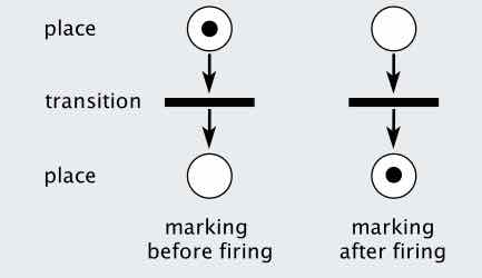mutex token) is a clean, minimal picture of exactly the race-condition-prevention problem that shows up for real once this series gets to multitasking and scheduling.

The Trade-off That Runs Through Everything

Step back and chapters 2 through 6 tell one continuous story. Continuous dynamics gives you ODEs and actors; discrete dynamics gives you FSMs: two separate modeling languages, each with its own precise notions of causality, determinism, and stability. Hybrid systems weld the two together mode by mode, which is the actual shape of most real cyber-physical systems: a thermostat, an AGV, a bouncing ball. Composition shows that even wiring FSMs together, on their own, is full of easily-conflated semantics: synchronous versus several flavors of asynchronous, shared-variable races, hierarchy edge cases. And concurrent models of computation is the catalog of coherent, well-studied answers to “what does composition actually mean here” (synchronous-reactive, the dataflow family, Petri nets, and the timed models), each one trading expressiveness against analyzability: determinism, bounded memory, freedom from deadlock.

That trade-off, more expressive concurrency buys less analyzability, is the single idea most worth carrying out of this phase. SDF’s rigid firing rules buy you decidable bounded-buffer and deadlock guarantees that DDF and process networks give up in exchange for flexibility, and picking a model of computation is really just picking a point on that trade-off curve. It’ll come back directly once this series gets to real-time scheduling and mutual exclusion, where the exact same tension (analyzable-but-restrictive versus flexible-but-unpredictable) shows up again wearing an operating-system’s clothes instead of a modeling language’s.