Why Turbo Codes Work

The previous entry ended with a working miracle and an unanswered question. Berrou, Glavieux and Thitimajshima showed that parallel concatenation with iterative decoding reaches within a fraction of a decibel of Shannon; they did not really show why, and their seven-page conference paper left one puzzle hanging in the air. The constituent encoders must be recursive, yet a recursive encoder and its nonrecursive parent generate exactly the same set of codewords. Same code, same distance spectrum, wildly different behavior inside a turbo scheme. How can that be? Three years later, Benedetto and Montorsi’s “Unveiling Turbo Codes” supplied the missing theory, and that puzzle is precisely its central object of study. This page works through their machinery: weight enumerators, the uniform interleaver, the $N^{1-w_{\min}}$ interleaver-gain law, and the design rules that fall out of it, then closes with the one thing their bound cannot do and the tool (EXIT charts) that fills the gap.

Weight Enumerators and the Union Bound

Benedetto’s entire analysis rests on a bookkeeping object. For a systematic code with $N$ input bits, the input-redundancy weight enumerating function (IRWEF) is

$$A^{C}(W,Z) = \sum_{w,z} A_{w,z}\, W^{w} Z^{z}$$

where $A_{w,z}$ counts the codewords whose input (systematic) weight is $w$ and whose parity weight is $z$; the total codeword weight is $w+z$. Fixing the input weight gives the conditional enumerator $A^{C}_{w}(Z) = \sum_z A_{w,z} Z^z$. Splitting the weight into an input part and a parity part, rather than lumping them together as a classical weight enumerator would, is not a cosmetic choice: the interleaver is about to act on the input bits only, so input weight is the quantity the whole analysis will be conditioned on.

Feed the enumerator into the standard union bound for maximum-likelihood decoding on the binary-input AWGN channel and you get a bound on the bit error probability:

$$P_b \;\le\; \sum_{w} \frac{w}{N} \sum_{z} A_{w,z}\; Q\!\left(\sqrt{2\,(w+z)\,R\,\frac{E_b}{N_0}}\right)$$

The $w/N$ factor is what distinguishes this from a word-error bound: a codeword of input weight $w$, when mistaken for the transmitted one, corrupts $w$ of the $N$ information bits. Hold onto that factor; it contributes one power of $N$ to the final result. With the bound in hand, every question about turbo performance becomes a question about the coefficients $A_{w,z}$ at small total weight $w+z$, because at moderate-to-high SNR the smallest arguments of the $Q$-function dominate the sum.

There is an immediate obstruction. The enumerator of a parallel concatenated code depends on which interleaver you chose. There are $N!$ candidates, $N$ is tens of thousands, and no closed form exists for any particular one.

The Uniform Interleaver

Benedetto’s Definition 1 dissolves the obstruction by refusing to pick an interleaver at all. A uniform interleaver of length $N$ is a probabilistic device that maps an input word of weight $w$ to each of its $\binom{N}{w}$ distinct permutations with equal probability $1/\binom{N}{w}$. No such physical device exists; it is an averaging instrument, the analytical stand-in for “an interleaver chosen at random.”

Its payoff is enormous. Under uniform interleaving, what the second encoder sees is a uniformly random rearrangement of whatever the first encoder saw, so the two constituent encoders become statistically independent given the input weight $w$, and the joint enumerator of the parallel concatenation factorizes:

$$\boxed{\;A^{C_p}_{w,z_1,z_2} \;=\; \frac{A^{C_1}_{w,z_1} \cdot A^{C_2}_{w,z_2}}{\dbinom{N}{w}}\;}$$

The average performance over all $N!$ interleavers is now computable from the two constituent enumerators alone, each of which comes from a small trellis.

Why should an average be meaningful? Benedetto’s answer is the same existence argument that powers random-coding proofs: the average over all interleavers is achievable by at least one deterministic interleaver, so the uniform-interleaver bound is not a fiction about imaginary hardware; some real permutation does at least this well. Empirically the statement is much stronger: almost all randomly drawn interleavers land close to the average, which is why the abstraction predicts real designs so faithfully.

Weight Enumeration via the Transfer-Matrix Method

The factorization is only useful if constituent enumerators are easy to compute, and they are: they fall out of a transfer matrix on the encoder’s state diagram. For a convolutional encoder with $2^M$ states, define the $2^M \times 2^M$ matrix

$$\left[\mathbf{A}(W,Z)\right]_{s',s} = \begin{cases} W^{\,w(s',s)}\,Z^{\,z(s',s)} & \text{if } s' \to s \text{ is a valid transition}\\[2pt] 0 & \text{otherwise} \end{cases}$$

where $w(s',s)$ is the input weight of the transition and $z(s',s)$ the parity weight it emits. The trick is that matrix multiplication does exactly the enumeration you want: it sums over intermediate states while multiplying monomials, and multiplying monomials adds the exponents. So $\left[\mathbf{A}^N\right]_{s',s}$ enumerates every length-$N$ path from $s'$ to $s$, each tagged with its total input and parity weight, and for a terminated code the conditional enumerators of the equivalent block code are read directly from one entry:

$$A^{C}(W,Z) = \left[\mathbf{A}(W,Z)^N\right]_{0,0}$$

Benedetto relegates this to his Appendix, but it deserves to be worked once in full, because the whole pipeline (matrix, power, factorization, bound) fits in a few lines for a small code. Take the 2-state recursive systematic encoder $G(D) = \left[1,\ \tfrac{1}{1+D}\right]$ with block length $N=4$. The state is $s = a_{k-1}$, the recursion is $a_k = d_k \oplus a_{k-1}$, and the parity output is $p_k = a_k$. Enumerating the four transitions:

from $s$	$d_k$	$a_k$	parity	to $s$	monomial
0	0	0	0	0	$1$
0	1	1	1	1	$WZ$
1	0	1	1	1	$Z$
1	1	0	0	0	$W$

$$\mathbf{A}(W,Z) = \begin{pmatrix} 1 & WZ \\ W & Z \end{pmatrix}$$

Square it once:

$$\mathbf{A}^2 = \begin{pmatrix} 1+W^2Z & WZ+WZ^2 \\ W+WZ & W^2Z+Z^2 \end{pmatrix}$$

Square again and keep only the $(0,0)$ entry:

$$A^C(W,Z) = \left[\mathbf{A}^4\right]_{0,0} = (1+W^2Z)^2 + (WZ+WZ^2)(W+WZ) = 1 + W^2\!\left(3Z + 2Z^2 + Z^3\right) + W^4 Z^2$$

A sanity check is available because this encoder is so simple: its state after $N$ steps is just the parity of the inputs, so every even-weight input word returns to state 0 and is a valid terminated codeword. There are $\binom{4}{2} = 6$ weight-2 inputs, and indeed the $W^2$ coefficients sum to $3+2+1 = 6$; there is $\binom{4}{4} = 1$ weight-4 input, and the $W^4$ term is a single monomial. The machine is counting correctly.

Now build the rate-1/3 PCCC from two copies of this encoder joined by a uniform interleaver of length 4. The factorization says to multiply the two conditional enumerators (squaring, since the encoders are identical; the product convolves the two parity weights, so the exponent of $Z$ becomes the total parity $z_1 + z_2$) and divide by $\binom{N}{w}$. For $w=2$:

$$A^{C_p}_2(Z) = \frac{\left(3Z+2Z^2+Z^3\right)^2}{\binom{4}{2}} = \frac{9Z^2+12Z^3+10Z^4+4Z^5+Z^6}{6} = \tfrac{3}{2}Z^2 + 2Z^3 + \tfrac{5}{3}Z^4 + \tfrac{2}{3}Z^5 + \tfrac{1}{6}Z^6$$

Those fractional coefficients are the signature of the uniform interleaver, and they are what Benedetto’s Example 2 is exhibiting: they are not counts of codewords (no code has one and a half codewords of weight 4) but averages over all $4!$ permutations. Some interleavers give this PCCC two codewords with $w=2,\,z=2$; most give one or none; the mean is $3/2$. The lowest-order term tells you the toy code’s effective distance: the minimum total weight reachable from a weight-2 input is $2+2 = 4$. Feed $A^{C_p}_w(Z)$ into the union bound above and you have the complete interleaver-averaged performance curve of a turbo code, computed from nothing but a $2\times2$ matrix. Everything Benedetto plots is this pipeline run on bigger constituents.

Derivation of the Interleaver Gain Exponent

Now for the theorem the whole paper exists to prove. Recall the fact the previous entry established on the trellis: because a recursive encoder’s feedback polynomial sits in the denominator of its transfer function, its impulse response is infinite, so a weight-1 input sets the register cycling forever and never produces a finite-weight error event. Define $w_{\min}$ as the smallest input weight that can produce a finite-weight error event. For a recursive encoder $w_{\min} = 2$; for a nonrecursive encoder, whose impulse response is finite, $w_{\min} = 1$.

Benedetto’s equation (20) turns that single integer into an asymptotic law, and the derivation is a counting argument short enough to give completely. Let $N_{w_{\min}}$ be the number of minimum-weight error events per unit time in the constituent code, and count how weight-$w_{\min}$ inputs fare in a length-$N$ turbo code.

First, count the bad patterns for encoder 1. An error event occupies a short, fixed span of trellis and can begin at any of roughly $N$ time instants, so about $N \cdot N_{w_{\min}}$ input sequences of weight $w_{\min}$ drive encoder 1 into a minimum-weight event. Second, count all patterns: there are $\binom{N}{w_{\min}} \approx N^{w_{\min}}/\,w_{\min}!$ input sequences of weight $w_{\min}$ in total. Third, ask the interleaver for its verdict. Under uniform interleaving the permuted sequence is equally likely to be any weight-$w_{\min}$ sequence, so the probability that encoder 2 is also driven into a low-weight event is the ratio of the first count to the second:

$$\Pr[\text{both bad}] \;\approx\; \frac{N\,N_{w_{\min}}}{N^{w_{\min}}/\,w_{\min}!} \;=\; w_{\min}!\;N_{w_{\min}}\; N^{\,1-w_{\min}}$$

Fourth, the expected number of low-weight PCCC codewords is (bad patterns for encoder 1) times (probability encoder 2 cooperates), which scales as $N \cdot N^{1-w_{\min}} = N^{\,2-w_{\min}}$. Fifth and finally, convert to a bit error contribution: the union bound weights each codeword by $w/N = w_{\min}/N$, spending one more power of $N$:

$$\boxed{\;\text{error coefficient} \;\propto\; \frac{w_{\min}}{N}\cdot N^{\,2-w_{\min}} \;=\; w_{\min}\, N^{\,1-w_{\min}}\;}$$

Substituting the two values of $w_{\min}$ produces the punchline of the paper:

Constituent code	$w_{\min}$	Coefficient scaling	Verdict
Recursive (RSC)	2	$N^{-1}$	coefficient shrinks as $1/N$: interleaver gain
Nonrecursive (NSC)	1	$N^{0}$	no gain at all; performance independent of $N$
Block codes (PCBC)	1	$N^{0}$	no gain; why parallel concatenated block codes underperform

A recursive constituent code lets the interleaver convert sheer length into a $1/N$ suppression of the error coefficient. A nonrecursive one gets nothing: you can grow the interleaver from a hundred bits to a million and the bound does not move. The same failure afflicts parallel concatenations of block codes, which is why the turbo construction is specifically a convolutional, recursive story.

The Role of Recursive Encoding

Here is the resolution of the puzzle from the opening, and it is the most conceptually interesting thing in the paper. A recursive encoder and its nonrecursive parent with the same transfer function generate exactly the same set of codewords: same code, same distance spectrum, and, used alone with ML decoding, essentially the same performance. Benedetto’s Figure 19 makes the point brutally by simulating both as ordinary standalone codes: the curves nearly coincide, and above 1 dB the nonrecursive one is actually slightly better. What differs is the input-to-codeword mapping: which input sequence gets assigned to which codeword. Recursion reshuffles that assignment so that the dangerous low-weight codewords require input weight 2 rather than input weight 1 to reach, and the mapping, not the codeword set, is what the interleaver acts on. Benedetto singles this out as the analysis’s single most important qualitative fact: recursive and nonrecursive constituent codes perform the same alone, and completely differently inside a parallel concatenation. Recursion, in other words, is not a property of the code at all. It is a property of the encoder, and turbo codes are the case in coding theory where the encoder matters independently of the code it generates.

His Figures 20 and 21 show the mechanism pictorially. For the recursive encoder, low-weight inputs produce parity weights spread broadly and roughly uniformly across the whole range; for the nonrecursive encoder, low-weight inputs concentrate on a small set of low parity weights, and when those convolve with themselves in the concatenation the resulting spectrum is poor. The rest of his experimental section fills in the quantitative picture:

Experiment	Setup	Finding
Interleaver gain (Fig. 22, D/E)	recursive constituents, $N=100$ vs $1000$	about 3 dB of gain from the $10\times$ longer interleaver
Same, nonrecursive (Fig. 22, B/C)	nonrecursive constituents, $N=100$ vs $1000$	essentially no change; confirms $N^{0}$
$N=1$ edge case (B vs D)	no interleaving at all	the nonrecursive PCCC wins, since duplicated parity gives it larger free distance
Constituent size (Fig. 15)	rate-1/3, 2 to 16 states	more states give better $d_{\text{eff}}$ and a steeper floor
Bound vs simulation (Fig. 17)	increasing decoder iterations	simulated curves converge progressively onto the ML union bound

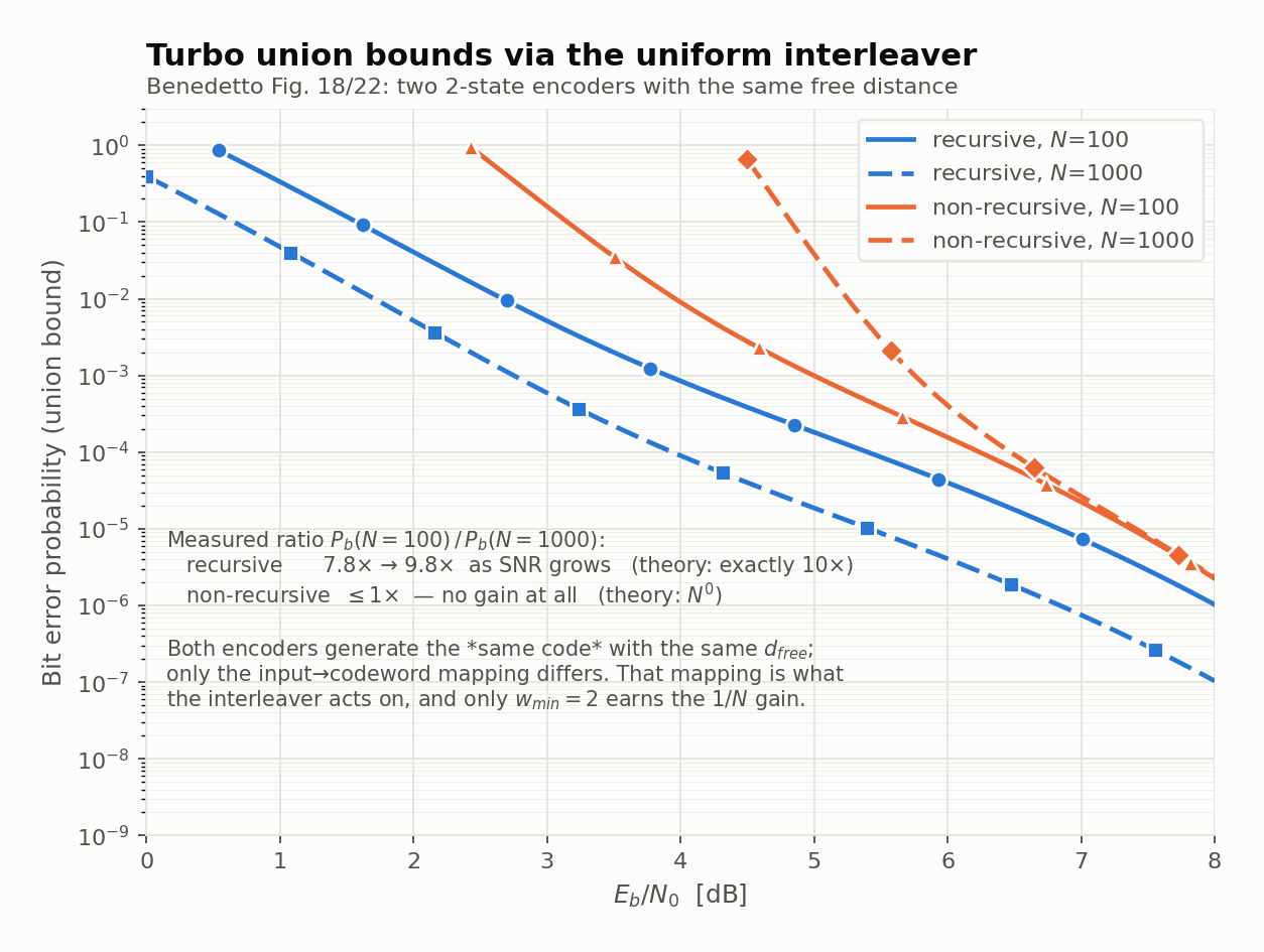The figure above runs the exact computation for the very encoder pair Benedetto used to make the argument, and the $1/N$ prediction lands within two percent. Note what the nonrecursive curves are quietly telling you: they are not merely failing to improve, they are pinned by codewords the interleaver cannot dilute.

The bound is one thing and a real decoder is another, so it is worth checking that an actual iteratively decoded turbo code behaves the way the theory says. Simulating a rate-1/3 code at three interleaver lengths, with eight iterations of log-MAP decoding at each: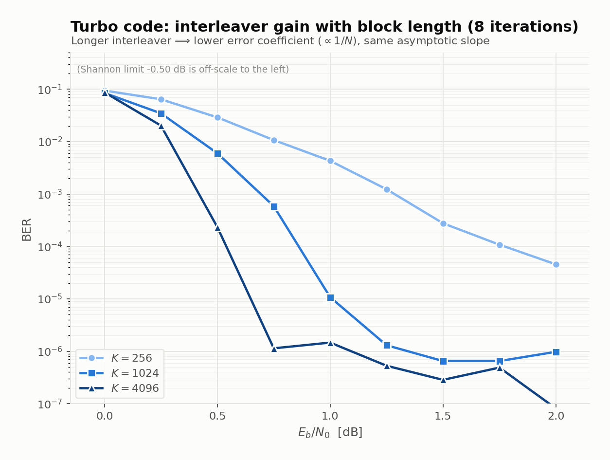

Read it against the boxed law and the agreement is structural rather than approximate. Lengthening the interleaver moves each curve down, which is the error coefficient shrinking as $1/N$, and it does so by a roughly constant factor per fourfold increase in $K$, exactly as a power law demands. What lengthening the interleaver conspicuously does not do is change how steeply the curves fall, because the slope is set by $d_{\text{eff}}$ and $N$ never enters the $Q$-function. This is the practical payoff of the whole analysis: the interleaver is the knob for the height of the error floor and the constituent code is the knob for its slope, and the two are independent.

Design Guidelines

Combine the interleaver-gain law with the union bound and keep only the dominant weight-2 term. For a recursive-constituent PCCC at large $N$,

$$P_b \;\approx\; \frac{c}{N}\; Q\!\left(\sqrt{2\, d_{\text{eff}}\, R\, \frac{E_b}{N_0}}\right)$$

where $d_{\text{eff}}$, the effective free distance, is the minimum total codeword weight over weight-2 inputs. This formula is the turbo designer’s entire dashboard, and it has exactly two knobs.

The first knob is $N$. Lengthening the interleaver buys the $1/N$ coefficient directly: cheap in performance, expensive in latency, since nothing can be decoded until the whole block arrives. Berrou used $N = 65536$; his reference chip design accepted 2318 bits of latency for a far smaller configuration. And there is a second, structural cost hiding behind the first: the BCJR decoder’s backward recursion cannot even begin until the entire block has been received, a serialism that seems like a footnote now but becomes the decisive liability when this series reaches the hardware race in the finale.

The second knob is $d_{\text{eff}}$, and it is set by the choice of constituent code, specifically the feedback polynomial. You want weight-2 inputs to generate as much parity weight as possible before the register returns to zero, and the register returns to zero only when the second 1 arrives a multiple of the state-cycle period after the first. A primitive feedback polynomial of degree $m$ maximizes that period at $2^m - 1$, forcing the surviving weight-2 events to be as long, and as parity-heavy, as possible. The rule of thumb “use primitive feedback” is this argument compressed to four words.

Notice what is not on the dashboard. The constituent code’s own free distance $d_{\text{free}}$ never appears, and $d_{\text{eff}}$ can be much larger than it. The 4-state RSC(7,5) from the previous entry has $d_{\text{free}} = 5$, achieved by a weight-3 input; but weight-3 events are crushed by $N^{-2}$ scaling, so the quantity that survives is the weight-2 figure $d_{\text{eff}} = 2 + 4 + 4 = 10$ for the rate-1/3 PCCC, double the free distance and attached to a different input weight entirely. Hence Forney’s remark: “Turbo codes seem to turn the conventional design principles on their head; they make error coefficients more important than minimum distance!”

Two misconceptions dissolve under the same light. First, turbo codes are emphatically not good because their constituent codes are good: the constituents are deliberately weak, 4 to 16 states, and at a fixed complexity budget stronger constituents actually hurt, because the strength lives in $N$ and the iteration, not in the trellis. Second, interleaver gain does not mean a longer interleaver improves the distance. It improves the coefficient, $N^{1-w_{\min}}$, and nothing else: $N$ appears in front of the $Q$-function and never inside it, so the asymptotic slope of the curve is set by $d_{\text{eff}}$ alone and is independent of $N$. Benedetto notes explicitly that curves for different interleaver lengths eventually merge as SNR grows. Length moves the floor down; it does not tilt it.

Error Floor and Interleaver Design

The $1/N$ gain reduces the number of low-weight codewords but does not eliminate them, and at high SNR the survivors dominate. The result is the error floor: the BER curve falls steeply through the waterfall, then flattens onto the gentle slope set by $d_{\text{eff}}$, typically around $10^{-6}$ to $10^{-7}$ for a naive interleaver.

The surviving bad codewords have a precise anatomy. Take a weight-2 input whose two 1s are separated by a multiple of the cycle period, so encoder 1 produces a short, low-weight parity burst. Usually the interleaver scatters those two positions and encoder 2 sees a high-weight event; the floor comes from the unlucky patterns whose images under the permutation are also separated by a multiple of the period, so both encoders emit low-weight parity simultaneously. Interleaver design is the art of making such doubly-bad patterns impossible rather than merely improbable:

Interleaver	Idea	Effect
Block (row-column)	Berrou’s $256 \times 256$ array	simple but poor; the regular structure mass-produces bad patterns
Pseudo-random	one uniform random permutation	good on average, occasional bad instance
S-random	reject $\pi(i)$ if $\lvert\pi(i)-\pi(j)\rvert < S$ whenever $\lvert i-j\rvert < S$	guarantees nearby bits stay apart, killing the short weight-2 patterns
ARP / QPP	algebraic, contention-free permutations	same performance, parallelizable in hardware; LTE adopted QPP

The other floor contributor is trellis termination. An RSC encoder cannot be driven to the zero state by appending zeros the way a nonrecursive encoder can: the feedback keeps the register cycling, which is the same fact that made $w_{\min}=2$ in the first place. Termination requires feeding the register contents back into the input for $M$ steps. In practice designers often terminate encoder 1 and leave encoder 2’s trellis open, in which case the second decoder’s backward recursion must start from a uniform distribution over final states, admitting ignorance: a small but real loss, and another entry on the floor’s ledger.

Limitations of the Union Bound

It is worth being precise about the epistemic status of everything above, because the bound has sharp limits and Benedetto is honest about all of them. First, it is a union bound on maximum-likelihood decoding, and iterative turbo decoding is not ML; strictly, it bounds the wrong decoder. Second, like every union bound it diverges below the cutoff rate, which is exactly the waterfall region where turbo codes earn their fame: the bound is structurally silent about the one thing everyone wanted explained in 1993. What it does deliver is the high-SNR story: there the bound is tight, and it predicts the error floor accurately, which is why everything in the previous two sections is trustworthy engineering rather than heuristics.

The bridge between the two decoders is empirical. Benedetto’s Figure 17 overlays simulated iterative-decoding curves on the ML bound and shows them converging onto it as the iteration count grows, the strongest evidence in the paper that iterative decoding is asymptotically ML-like. Whether it truly converges to ML is listed, with commendable candor, as open problem number one in his concluding section.

EXIT Chart Analysis

So the waterfall needed a different tool, and turbo codes eventually got one: not an exact analysis but a remarkably effective semi-empirical one, ten Brink’s EXIT charts (1999). The starting point is an observation Berrou himself had already published without pursuing: his Figure 6 shows the histogram of the extrinsic values starting decidedly non-Gaussian at iteration 1 and converging toward a Gaussian with mean $\pm1$ as iterations progress. EXIT analysis promotes that observation to a modeling assumption. Take the extrinsic LLRs to be Gaussian and consistent, meaning the symmetry of correct LLRs locks the variance to the mean:

$$L_e \sim \mathcal{N}(\mu,\,\sigma_e^2) \quad\text{with}\quad \sigma_e^2 = 2\mu$$

so a single scalar describes the entire message distribution. Rather than tracking $\mu$ directly, ten Brink tracks the mutual information $I \in [0,1]$ between a bit and its LLR, computed from the Gaussian model via

$$J(\sigma) \;=\; 1 - \int_{-\infty}^{\infty}\frac{1}{\sqrt{2\pi\sigma^2}}\; e^{-\frac{(\xi-\sigma^2/2)^2}{2\sigma^2}}\,\log_2\!\left(1+e^{-\xi}\right)d\xi$$

which is monotonic, hence invertible, and in practice tabulated once. The mutual-information coordinate is the robust choice: it saturates sensibly at 0 and 1 and is far less sensitive to the Gaussian idealization than the raw mean would be.

Each constituent decoder is then characterized, by simulation, exactly once: feed it synthetic a priori LLRs drawn from the consistent Gaussian with a priori information $I_A$, run it at a given $E_b/N_0$, and measure the mutual information $I_E$ of its extrinsic output. The result is a transfer characteristic $I_E = T(I_A,\, E_b/N_0)$, one curve per decoder per SNR. Plot decoder 1’s curve on axes $(I_{A1}, I_{E1})$ and decoder 2’s curve on the same axes with its coordinates swapped, which is legitimate because one decoder’s extrinsic output is the other’s a priori input. Iterative decoding then traces a staircase between the two curves:

Reading the chart is reading the decoder’s fate. If the tunnel between the curves is open, the staircase climbs all the way to $(1,1)$: decoding converges, and the number of steps predicts the number of iterations needed. If the curves pinch together, the staircase jams at the fixed point and decoding stalls; the SNR at which the tunnel first closes is the convergence threshold, the quantity Benedetto’s bound could never reach. A tunnel that is open but narrow means convergence only after many iterations, which is precisely the steep “turbo cliff” seen in simulation. And the chart is a design tool, not just a diagnostic: you want the two transfer curves well matched, hugging each other with minimal enclosed area, because tunnel area is wasted SNR. Curve matching became the design principle of the iterative-decoding era. Keep that phrase in mind, along with a forward echo worth planting now: everything in this section is an approximation resting on one Gaussian assumption, and the next family of codes in this series comes with an exact version of the same fixed-point analysis.

Check Yourself

1. Why must the constituent encoders of a turbo code be recursive?
2. State the definition of the uniform interleaver and what it buys the analysis. Why is a bound computed with it meaningful for real systems?
3. A constituent code has $d_{\text{free}} = 7$, achieved by a weight-3 input, and its weight-2 inputs produce minimum parity weight 6. What is $d_{\text{eff}}$ of the rate-1/3 PCCC built from two copies of it?
4. You double the interleaver length from 1024 to 2048. What happens to the error floor’s height? To its slope?
5. Your colleague uses Benedetto’s union bound to predict the SNR at which a new turbo code’s waterfall begins. What do you tell them, and what tool should they use instead?

Answers

1. Only a recursive encoder has $w_{\min} = 2$: its infinite impulse response means a weight-1 input never produces a finite-weight error event. The error coefficient scales as $N^{1-w_{\min}}$, so $w_{\min}=2$ yields $1/N$ interleaver gain while a nonrecursive encoder’s $w_{\min}=1$ yields none. The codeword set is identical either way; what differs is the input-to-codeword mapping, and the interleaver acts on the mapping.

2. A probabilistic device mapping each weight-$w$ input word to all $\binom{N}{w}$ of its permutations with equal probability. It makes the two constituent encoders conditionally independent given $w$, so the PCCC enumerator factorizes as $A^{C_1}_{w,z_1}A^{C_2}_{w,z_2}\big/\binom{N}{w}$, and the interleaver-averaged performance becomes computable from the constituent enumerators alone. The average is meaningful because at least one deterministic interleaver achieves it, and empirically almost all of them come close.

3. $d_{\text{eff}} = 2 + 6 + 6 = 14$: systematic weight 2 plus the minimum weight-2 parity from each encoder. The $d_{\text{free}} = 7$ figure is a distractor; it belongs to a weight-3 input, and weight-3 events are suppressed as $N^{-2}$, so they do not set the floor.

4. The height drops by a factor of 2 (the $1/N$ coefficient), roughly 3 dB in the floor. The slope is unchanged: it is set by $d_{\text{eff}}$, which does not depend on $N$, and $N$ never enters the $Q$-function. Curves for different $N$ eventually merge at high enough SNR.

5. The union bound diverges below the cutoff rate, so it is structurally incapable of predicting the waterfall; it is a high-SNR tool that predicts the error floor. For the waterfall they need a convergence analysis of the iterative decoder itself: an EXIT chart, finding the SNR at which the tunnel between the two decoders’ transfer characteristics opens.

Where This Leaves Us

Benedetto and Montorsi turned Berrou’s astonishing experiment into engineering. The uniform interleaver made the average analyzable; the transfer-matrix pipeline made it computable; the counting argument produced the $N^{1-w_{\min}}$ law; and the law answered the planted question with a genuinely deep observation, that recursion is a property of the encoder rather than the code, and the interleaver rewards the encoder’s mapping, not the code’s distances. Out of it fell the working design rules (grow $N$ for the coefficient, choose primitive feedback for $d_{\text{eff}}$, engineer the interleaver against doubly-bad weight-2 patterns) and an honest boundary: the bound owns the floor, EXIT charts watch the waterfall, and neither is an exact theory of the iterative decoder.

Meanwhile the turbo shock had a second consequence, sociological rather than mathematical. It sent researchers back through the literature hunting for anything else that iterated soft information on a random-looking structure, and MacKay and Neal found exactly that waiting in a thesis from 1962: Gallager’s sparse-graph codes, complete with an iterative decoder nobody had been able to afford. Their rediscovery comes with the payoff foreshadowed above: where turbo analysis leans on a Gaussian assumption, LDPC codes admit an exact fixed-point analysis of the decoder itself, density evolution, and it is the subject of the next entry.