Instruction Sets & Processor Architecture

Phase 1 stayed almost entirely abstract (actors, state machines, models of computation) without asking what any of it actually runs on. This phase grounds that abstraction in real hardware: two concrete instruction sets from Wolf’s book, ARM and the TI C55x DSP, and the conceptual apparatus Lee and Seshia supply for reasoning about any embedded processor you might encounter.

Two Design Philosophies: von Neumann vs. Harvard, RISC vs. CISC

Before looking at any specific chip, it’s worth having the two big axes of variation in hand. The first is about memory: a von Neumann machine uses one shared memory for both data and instructions; a Harvard machine keeps them in separate memories with separate ports. Harvard wins specifically for DSPs, because streaming data needs high, predictable memory bandwidth, and two independent ports mean data fetches and instruction fetches never have to compete for the same bus. Most DSPs are Harvard machines; among ARM chips, ARM7 is von Neumann and ARM9 is Harvard, a distinction that’s completely invisible to someone writing assembly, and only shows up as a difference in performance.

The second axis is about the instruction set itself: RISC favors fewer, simpler, uniform-length instructions chosen specifically so they pipeline efficiently; CISC allows richer, variable-length instructions with fewer restrictions: a single instruction that does a string search, say. RISC’s early performance advantage over CISC has narrowed over time, mostly because RISC-style execution techniques turn out to handle a common CISC subset efficiently too.

One more distinction is worth having precise before diving into ARM and the C55x: a programming model (the register set visible to the programmer) is defined by the architecture, but a single instruction-set architecture (ISA) can have many different silicon realizations, with different clock speeds, caches, and buses. Same instructions, different non-functional behavior. Lee and Seshia flag the trap this creates directly: an ISA carries no timing guarantees at all, so “runs correctly on chip A” says nothing about whether the same code meets its deadlines on chip B.

ARM: A Concrete Load-Store RISC

ARM is a load-store architecture: ALU operations only ever touch registers, never memory directly, so data has to be 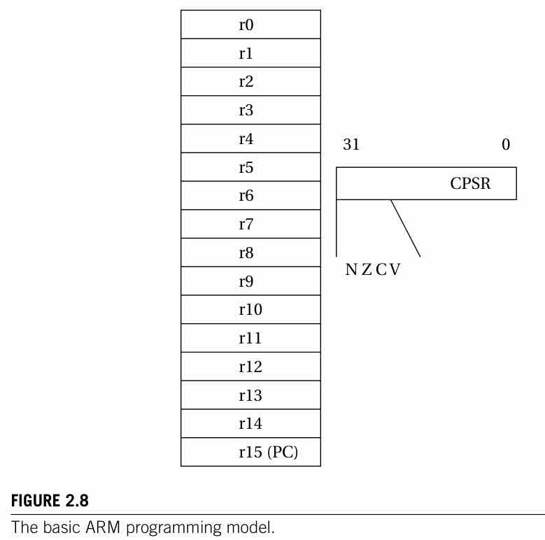LDR’d in and STR’d back out explicitly. It has 16 general registers, r0 through r15, where r15 doubles as the program counter and r14 holds the return address after a BL (branch-and-link) instruction.

The CPSR (current program status register) automatically updates its N/Z/C/V flags on every arithmetic or logical operation, and ARM does something distinctive with them: every instruction, not just branches, can execute conditionally by testing these flags: a genuinely different way to implement if-like logic that doesn’t always require an actual branch. Its addressing modes, register, immediate, register-indirect ([r1]), base-plus-offset ([r1,#16]) with auto-indexing (updating the base before use) or post-indexing (updating it after), are exactly the family that makes array and loop code, and stack push/pop, compact to write. And because a full 32-bit address can’t fit inside a 32-bit instruction word, ARM generates addresses via PC-relative arithmetic (the ADR pseudo-op) rather than loading one directly.

A few control-flow patterns are worth internalizing here because they’re the general RISC pattern, not something specific to ARM: conditional branches implement if; a branch table (an array of code addresses, indexed and jumped to via a single LDR into the program counter) implements switch far more efficiently than a chain of compares; BL saves a return address in the link register, good for one level of call depth; and the moment calls start nesting, you need a software-maintained call stack: push the return address, arguments, and saved registers on entry, pop them on exit. That’s the actual reason every CPU with subroutines needs a stack convention, not a quirk of ARM’s.

The TI C55x: A DSP Built for One Job

Where ARM is general-purpose, the C55x is built around one computational pattern and nothing else. It’s an accumulator architecture, not a general-purpose-register one: almost all arithmetic looks like accumulator ← operand ⊕ accumulator, which matches the DSP-native sum-of-products pattern $a_1x_1 + a_2x_2 + \cdots$ exactly. There are four 40-bit accumulators (32 data bits plus 8 guard bits giving headroom across long chains of multiply-accumulate before you have to normalize), a width that’s deliberately over-provisioned compared to ARM’s uniform 32-bit registers.

Registers here are specialized rather than uniform: separate registers exist for loop-repeat counts, circular-buffer bounds, coefficient pointers, and interrupt masks. That’s a direct hardware reflection of what DSP code actually looks like (tight arithmetic loops over streaming data), the opposite design philosophy from ARM’s general-purpose regularity. Addressing modes are correspondingly narrow: just three (absolute, direct, indirect) against ARM’s much richer set, because DSPs trade addressing generality for extreme efficiency on the one loop shape (the tapped delay line, or circular buffer) that dominates their workload. The takeaway generalizes well beyond these two chips: every CPU reads and writes memory, does arithmetic, and branches, but how an architecture specializes its registers, addressing, and instructions is a direct signature of the workload it was built for. ARM optimizes for general, control-flow-heavy code; the C55x optimizes for one specific kind of numeric inner loop.

What Makes a DSP a DSP

Embedded computing has no single dominant ISA the way x86 dominates desktop machines: designers choose from microcontrollers (small, cheap, low-power, often 8-bit), DSPs, GPUs, and increasingly heterogeneous multicore SoCs, picking whichever fits the workload. Lee and Seshia’s chapter gives a precise answer to what actually makes something a DSP, rather than the fuzzier “does signal processing”: to qualify, a processor has to execute one FIR filter tap (one multiply-accumulate plus two address updates) in a single instruction cycle. Everything else associated with DSPs (Harvard memory, a hardware MAC unit, circular-buffer or bit-reversed addressing, wide accumulators) exists purely to make that one guarantee hold.

The FIR filter is worth understanding structurally, because it’s the canonical signal-processing computation and recurs constantly, both in DSP hardware design and later in filtering and estimation topics. It’s a weighted sum of the $N$ most recent input samples:

$$y(n) = \sum_{i=0}^{N-1} a_i \, x(n-i)$$

where $x(n)$ is the input stream, the $a_i$ are the filter’s tap coefficients, and $y(n)$ is the output. The natural hardware realization is a tapped delay line: each new sample shifts down a chain of unit-delay elements, each tap gets scaled by its coefficient, and the products sum to the output.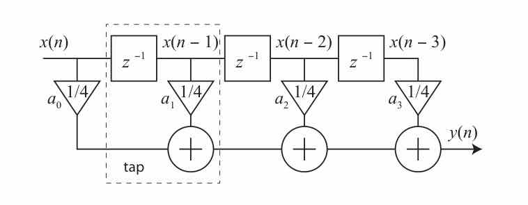

Implementing that delay line by physically shifting data in memory every sample would be wasteful, so DSPs use a circular buffer instead (a ring-indexed array with modulo pointer arithmetic), which is exactly why they bake hardware modulo-addressing support into their auxiliary registers. The single instruction that makes one FIR tap execute per cycle is the MAC (multiply-accumulate):

$$a \leftarrow a + x \cdot y$$

where $a$ is an accumulator and $x, y$ are operands fetched via auto-incrementing, often circular, address registers: two memory fetches, a multiply, an add, and two address increments, all in one instruction cycle on real hardware.

Lee and Seshia also draw a distinction in this chapter that’s easy to blur and worth being precise about: concurrency is not parallelism. Concurrent means conceptually simultaneous (a property of the program’s logic); parallel means physically simultaneous (a property of the actual execution). A multitasking OS can run a concurrent program entirely sequentially, interleaved, and superscalar or VLIW hardware can then execute that same sequential instruction stream in parallel again: two independent translations stacked on top of each other, which is exactly why reasoning precisely about real-time timing gets hard. There’s a sharper, CPS-specific version of this point worth keeping: for embedded systems, concurrency isn’t primarily about speed at all. Physical processes are inherently concurrent (multiple sensors, multiple actuators, all happening at once in real time), so a program’s concurrency mirrors the physical problem’s concurrency, not just a performance optimization. Finishing early isn’t automatically better, either: a spark plug fired early is exactly as wrong as one fired late. The correctness criterion is timeliness, not throughput.

Pipelines, Hazards, and the Cost of Speed

A standard processor pipeline has five stages (fetch, decode, execute, memory, writeback), with latches between stages letting five instructions be in flight at once. A reservation table (a resource-by-cycle grid) is the right way to visualize exactly which instruction is occupying which hardware unit on any given cycle.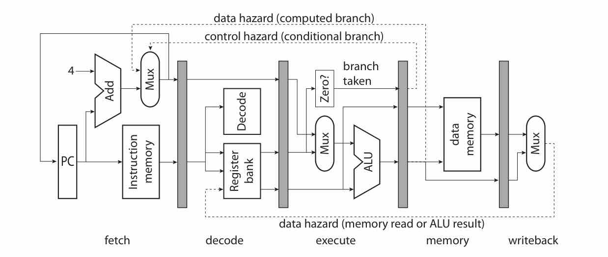

Two kinds of hazard show up once instructions overlap this way. A data hazard happens when instruction B reads a register that instruction A (still in flight, not yet at writeback) is about to write, so B risks reading a stale value; fixes range from an explicit pipeline (the compiler inserts NOP bubbles and the hazard is the programmer’s problem) to interlock (hardware stalls B automatically) to forwarding (hardware routes A’s result straight to B without waiting for the actual write) to out-of-order execution (hardware reschedules independent later instructions ahead of the stalled one), each step trading more hardware complexity for less programmer burden. A control hazard happens because a conditional branch’s target isn’t known until a later pipeline stage, but the pipeline has already speculatively fetched whatever comes next sequentially; fixes here are a delayed branch (the compiler fills the delay slot with something safe), interlock again, or speculative execution (guess, then roll back any register writes if the guess was wrong).

The consequence that matters most for embedded work: everything past the simplest fixes (explicit pipelines, delayed branches) makes instruction timing variable, harder to predict, and in the extreme case of superscalar out-of-order execution, not even repeatable from one run to the next. That’s exactly why DSPs favor simple, explicit pipelines, where precise and analyzable timing matters more than raw throughput, while general-purpose CPUs favor out-of-order and speculative execution, where aggregate throughput matters more than any single instruction’s exact timing.

More Parallelism, Less Predictability

There’s a spectrum of instruction-level parallelism, and it’s ordered by a clear trend: more hardware autonomy, less programmer or compiler control, in this order: CISC instructions, where one instruction packs in many primitive operations (a MAC is two fetches, a multiply, an add, and two modulo-increments, all in one cycle); subword parallelism, splitting a wide ALU into narrow lanes for something like four 8-bit pixel-channel operations at once, a restricted form of vector processing; superscalar, where hardware discovers independent instructions at runtime and dispatches, even reorders, them in parallel, buying great average throughput at the cost of poor timing predictability, since timing can end up depending on exactly where an interrupt happens to land; and VLIW, where the compiler or programmer statically decides what runs in parallel each cycle and encodes that directly into the instruction, less flexible, but the resulting timing is repeatable. VLIW is generally the better fit for embedded and real-time work precisely because superscalar’s dynamic scheduling trades predictability for average-case speed, and that’s the wrong trade when correctness depends on a deadline.

Multicore designs split the same way: homogeneous multicore repeats identical cores; heterogeneous multicore mixes core types on one die: the TI OMAP pairing an ARM core for UI and networking with a DSP core for radio and media is the standard example. Heterogeneous multicore is attractive specifically because a hard-real-time task, like radio protocol timing, can get a dedicated core, immune to interference from whatever a general-purpose task is doing on another core, with one real caveat: a shared higher-level cache across cores reintroduces exactly that interference, since one core’s cache misses can evict another core’s working set, which is why shared multi-level caches are a poor fit for real-time cores. Soft cores on FPGAs are the other path into multicore: a processor synthesized directly in reprogrammable logic, easy to couple tightly to custom, application-specific hardware sitting right next to it.

Fixed-Point Arithmetic: Doing Fractions Without a Float Unit

Most embedded and DSP hardware has no floating-point unit at all, so non-integer values are represented as fixed-point: an ordinary integer with an imagined binary point at a fixed position, written as format n.m: $n$ bits before the point, $m$ after. This is purely a software convention; the hardware underneath is just doing plain integer math. The law of conservation of bits follows directly from that: multiplying an n.m value by a p.q value produces an (n+p).(m+q) result (two 1.15 values multiply out to a 2.30 result), which is exactly why accumulators, like the C55x’s 40-bit ACx registers, are built roughly twice the width of ordinary data registers.

Packing a wide multiplication result back into a narrower register forces a real choice about which bits to keep, and both directions carry genuine numerical risk. Discarding a high-order bit can flip the sign outright ($-1 \times -1$ in 1.15 format literally overflows, because $+1$ isn’t representable in that format at all), and dropping low-order bits is either truncation (just cutting them off) or rounding (adding a half-ULP bias first). Neither is an incidental detail; both are numerical-correctness concerns a programmer has to actively manage.

Where This Leaves Us

Wolf’s ARM and C55x walkthroughs give two concrete, contrasting instruction-set philosophies (ARM’s regular load-store RISC register file against the C55x’s specialized accumulator-and-circular-buffer DSP design), and Lee and Seshia’s chapter supplies the conceptual apparatus for reasoning about any embedded processor: ISA versus realization, concurrency versus parallelism, pipeline hazards and how they get resolved, the ILP spectrum from CISC through VLIW, heterogeneous multicore, and fixed-point arithmetic as the standard workaround for missing floating-point hardware.

The recurring theme, again, is a predictability-versus-throughput trade-off: DSPs and VLIW favor precise, analyzable timing; general-purpose superscalar favors average-case speed at the cost of predictability. That’s central to picking a processor for a real-time embedded application, and it’s exactly the same tension (analyzable-but-restrictive against flexible-but-unpredictable) that resurfaces once this series reaches operating-system scheduling, where the question stops being “which instruction runs next” and becomes “which task runs next.”