LDPC Reborn: Density Evolution

The previous entry ended on an uncomfortable note: turbo codes work spectacularly, and the best available explanation (EXIT charts) is an approximation. The turbo shock of 1993 sent the whole field hunting for other codes that might respond to iterative decoding, and in 1996 MacKay and Neal found one sitting in the library: Gallager’s 1963 sparse-graph codes, reinvented, resimulated, and suddenly competitive with turbo. Then, in 2001, Richardson, Shokrollahi and Urbanke (RSU hereafter) gave LDPC codes the thing turbo codes never got: an exact asymptotic analysis. Their tool, density evolution, does not estimate the decoding threshold; it computes it, to as many digits as you care to run the numerics. The reason LDPC admits an exact theory while turbo does not is structural and worth stating up front. Density evolution needs the decoder’s incoming messages to be independent, which holds when the neighborhood of a node looks like a tree. A sparse random graph is locally tree-like: cycles exist, but they are long, and any fixed-depth view of the graph is cycle-free with probability approaching one as $n$ grows. The turbo graph is the opposite: two enormous structured cycles (the two trellises) threaded through an interleaver, tree-like nowhere. So turbo got EXIT charts, a Gaussian approximation; LDPC got a theorem. This page builds that theorem, uses it to design codes that landed 0.0045 dB from Shannon’s limit, and then walks the result back into the real world of encoders, standards, and the failure modes the theorem cannot see.

Irregular LDPC Code Ensembles

Gallager’s codes are regular: every variable node has the same degree $j$, every check node the same degree $k$. The first modern move, due to Luby and coauthors in the late 1990s, was to ask why. Suppose instead you give some variable nodes very high degree. A high-degree variable node collects evidence from many checks at once, so it converges fast and becomes reliable early. Once reliable, it feeds strong messages into every check it touches, and those checks in turn rescue their weaker, low-degree neighbors. An irregular graph is a bootstrapping structure: a well-connected core locks in first and pulls the periphery along behind it. The catch is conservation: the total edge count is pinned by the rate, so every high-degree variable node must be paid for with low-degree ones, and low-degree variable nodes are individually fragile. Where the optimal balance lies is a genuine optimization problem, and solving it is exactly what RSU’s paper does. But first the balance needs a notation.

RSU describe a degree profile by a pair of polynomials, and here is the warning that saves you the most grief on this entire page: these are edge-perspective distributions, not node-perspective ones. Write

$\lambda(x) = \sum_{i \ge 2} \lambda_i\, x^{i-1}, \qquad \rho(x) = \sum_{i \ge 2} \rho_i\, x^{i-1},$

where $\lambda_i$ is the fraction of edges attached to variable nodes of degree $i$, and $\rho_i$ the fraction of edges attached to check nodes of degree $i$. Both normalize, $\lambda(1) = \rho(1) = 1$. The trap is to read $\lambda_i$ as the fraction of nodes of degree $i$; it is not, because a degree-30 node soaks up thirty edges while a degree-2 node takes two, so high-degree nodes are heavily overrepresented in $\lambda$. If you need the node fractions, divide by degree and renormalize: the fraction of variable nodes of degree $i$ is $(\lambda_i/i)\big/\sum_{i'} \lambda_{i'}/i'$. Get this wrong and every rate calculation that follows comes out wrong.

Even the exponent is doing work. The polynomials use $x^{i-1}$, not $x^i$, and that is deliberate: a message leaving a node along one edge depends on the other $i-1$ edges at that node. This is the extrinsic principle you met in turbo decoding, and Gallager’s Theorem 4.1 before that, here baked directly into the notation so that the analysis formulas come out clean.

The rate follows from edge counting. Since $\sum_i \lambda_i/i$ is proportional to the number of variable nodes per edge, and likewise for checks, the design rate is

$\boxed{\;R \;=\; 1 - \frac{\int_0^1 \rho(x)\,dx}{\int_0^1 \lambda(x)\,dx}\;}$

(the integrals compute exactly those $\sum_i \lambda_i / i$ sums). Sanity-check it against the regular $(3,6)$ code, the running benchmark for this whole page: $\lambda(x) = x^2$ and $\rho(x) = x^5$, so $\int_0^1 \lambda = 1/3$ and $\int_0^1 \rho = 1/6$, giving $R = 1 - (1/6)/(1/3) = 1/2$, as it must.

Finally, the object of analysis is not a single code but an ensemble, in exactly Gallager’s methodological tradition: fix $n$ and $(\lambda, \rho)$, enumerate the edge sockets on the variable side and the check side, and match them by a uniformly random permutation. Every statement in the rest of this page is a statement about a code drawn at random from this ensemble; the next section explains why that is enough.

Foundations of the Analysis

Density evolution rests on three preparatory results, and it pays to state each one carefully, because each answers a specific objection you should be raising.

Step one: concentration. The obvious objection to ensemble analysis is that you will build one code, not an average. RSU’s concentration theorem answers it. Let $Z$ be the number of incorrect messages after $\ell$ iterations, for a code drawn at random from the ensemble and a random channel realization, and let $\bar z = \mathbb{E}[Z]/(n \bar d_v)$ be its normalized expectation. Then there is a constant $\beta > 0$, depending on $(\lambda,\rho)$ and $\ell$ but crucially not on $n$, such that for any $\varepsilon > 0$

$\Pr\left[\,\left|\tfrac{Z}{n \bar d_v} - \bar z\right| > \varepsilon\,\right] \;\le\; 2\,e^{-\beta \varepsilon^2 n},$

and separately the ensemble average itself converges to the cycle-free (“tree”) value $p_\ell$ with error at most $\gamma/n$. The proof of the first bound is an Azuma-Hoeffding martingale argument (expose the graph’s edges and the noise one item at a time; each exposure moves $Z$ by a bounded amount); the second is a direct count showing a depth-$2\ell$ neighborhood contains a cycle with probability $O(1/n)$. Chain the two statements together and you get the license for everything that follows: a random long code performs like the ensemble average, which performs like the tree value that density evolution computes, and each link in the chain carries a quantified error term. Analyzing the ensemble is analyzing your code.

Step two: the tree assumption. Fix the iteration count $\ell$ and let $n \to \infty$; then the depth-$2\ell$ neighborhood of a randomly chosen variable node is cycle-free with probability tending to one. On a tree, every incoming message to a node is statistically independent of every other, so the belief-propagation update is exact, and (this is the part that matters for analysis) the distributions of the messages compose by simple convolution. Now, the objection: any finite code has cycles, so the assumption is literally false for every code you will ever build. The resolution is that the tree assumption is never applied to a finite code. It is applied in the limit, where it holds; concentration then bounds how far a finite code can stray from the limit, and the deviation shrinks exponentially in $n$. Empirically the limit is an excellent guide: RSU simulate an $n = 10^6$ code and land 0.13 dB from capacity against a predicted threshold 0.06 dB from capacity. The threshold is the limit; finite length is the gap to it. Beware the shorthand “density evolution assumes a cycle-free code”; what it assumes is the ensemble average as $n \to \infty$, which is a different and defensible thing.

You can watch that gap close. Simulating the regular (3,6) ensemble at three block lengths, against its own density-evolution threshold of 1.11 dB: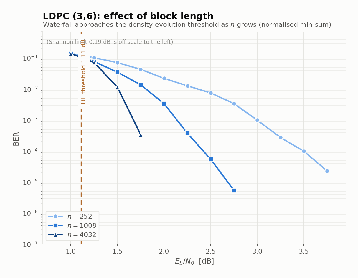

The threshold is a vertical line no finite code reaches, but the approach to it is orderly and visible. Lengthening the code does two things at once: it moves the waterfall toward the threshold, and it sharpens the waterfall into an actual cliff. Both are the concentration theorem made visual, since a longer code deviates less from the ensemble average and its neighborhoods are tree-like to greater depth. Note also what the asymptotic theory buys you in practice: having computed one number, 1.11 dB, from a cycle-free idealization, you know where the waterfall of a code you have not yet built will eventually sit.

Step three: symmetry, and the all-ones codeword. Tracking message distributions would still be hopeless if the answer depended on which codeword was sent. It does not, provided two symmetries hold. The channel must be output-symmetric, $p(y \mid x{=}0) = p(-y \mid x{=}1)$, and the decoder’s update rules must respect that symmetry; RSU’s Theorem 3 proves the belief-propagation updates preserve a precise density symmetry condition, $f(-x) = f(x)\,e^{-x}$, through every iteration. Under these conditions the conditional error probability is identical for every transmitted codeword, so you may analyze the most convenient one: the all-ones codeword in $\pm 1$ notation (equivalently the all-zeros codeword in bit notation). It is worth checking the symmetry condition once by hand for the channel that matters most. For BI-AWGN with unit amplitude and noise variance $\sigma^2$, the channel LLR is Gaussian with mean $\mu = 2/\sigma^2$ and variance $s^2 = 4/\sigma^2$; note $s^2 = 2\mu$, the consistency condition that will return in the Gaussian approximation. Then

$\frac{f(-x)}{f(x)} = \exp\!\left(-\frac{(x+\mu)^2 - (x-\mu)^2}{2 s^2}\right) = \exp\!\left(-\frac{4 x \mu}{2 \cdot 2\mu}\right) = e^{-x},$

exactly as required. With all-ones transmitted, the sign convention becomes wonderfully simple: a positive message is correct, a negative message is an error, and all of density evolution reduces to one question asked over and over: how much probability mass does the message density still have on the negative axis?

The Density Evolution Recursion

Now the construction itself. Write $P_0$ for the density of the channel LLRs, $Q_\ell$ for the density of variable-to-check messages at iteration $\ell$ (with $Q_0 = P_0$), and $R_\ell$ for the density of check-to-variable messages. The task is to compute $Q_\ell$ from $Q_{\ell-1}$, and it splits into an easy half and a hard half.

The easy half is the variable node. A degree-$i$ variable node sends out its channel LLR plus the sum of $i-1$ incoming check messages, and on the tree those summands are independent. The density of a sum of independent random variables is the convolution of their densities, so a degree-$i$ node emits $P_0 \circledast R_\ell^{\circledast(i-1)}$, where $\circledast$ is ordinary convolution on $\mathbb{R}$. To get the density on a randomly chosen edge, average over the edge-degree distribution, and here you see precisely why $\lambda$ was defined per edge rather than per node:

$Q_\ell \;=\; P_0 \circledast \sum_{i \ge 2} \lambda_i\, R_\ell^{\circledast(i-1)}.$

The hard half is the check node, because its update rule is multiplicative:

$\tanh\frac{L_{c \to v}}{2} \;=\; \prod_{v'} \tanh\frac{L_{v' \to c}}{2}.$

Densities do not compose under products, and you cannot rescue the situation by taking logarithms, because $\tanh(L/2)$ ranges over $[-1,1]$ and the factors can be negative. This is where RSU deploy the one genuinely clever trick in the whole construction: change coordinates so that the product becomes a sum. Split each message $m$ into a sign and a magnitude,

$m \;\longmapsto\; (s, r), \qquad s = \begin{cases} 0 & m \ge 0 \\ 1 & m < 0 \end{cases}, \qquad r = |m|,$

and handle the two parts separately. The sign part is immediate: the sign of a product is the product of the signs, and in $\{0,1\}$ notation a product of signs is an XOR, which is addition in $\mathrm{GF}(2)$. The magnitude part is where the logarithm becomes legal: taking absolute values gives $\tanh(r_{\text{out}}/2) = \prod_\ell \tanh(r_\ell/2)$ with every factor now in $(0,1]$, so apply $-\ln$ to both sides and define the magnitude map

$\gamma(r) \;\triangleq\; -\ln\tanh\frac{r}{2} \;=\; \ln\frac{e^r + 1}{e^r - 1},$

which maps $(0,\infty)$ to $(0,\infty)$ and turns the product into the sum $\gamma(r_{\text{out}}) = \sum_\ell \gamma(r_\ell)$.

The function $\gamma$ has a lovely property that halves your implementation work: it is an involution, $\gamma(\gamma(x)) = x$, so the transform is its own inverse. The proof takes three lines. Let $y = \gamma(x)$, so $e^y = \coth(x/2) = \frac{e^x + 1}{e^x - 1}$. Then

$\coth\frac{y}{2} = \frac{e^y + 1}{e^y - 1} = \frac{(e^x+1) + (e^x-1)}{(e^x+1) - (e^x-1)} = \frac{2e^x}{2} = e^x,$

so $\gamma(y) = \ln\coth(y/2) = x$. One function serves as both the forward and the inverse transform.

Assemble the pieces. Let $\Gamma$ denote the operator that pushes a density on $\mathbb{R}$ through $m \mapsto (\operatorname{sign} m,\, \gamma(|m|))$, producing a density on the group $\mathcal{G} = \mathrm{GF}(2) \times [0,\infty)$. Under $\Gamma$, the check-node operation is componentwise addition in $\mathcal{G}$, so densities compose by convolution over $\mathcal{G}$: XOR-convolution in the sign coordinate, ordinary convolution in the magnitude coordinate. Averaging over the check-degree distribution and transforming back,

$R_\ell \;=\; \Gamma^{-1}\!\left[\sum_{i \ge 2} \rho_i \left(\Gamma[Q_{\ell-1}]\right)^{\circledast_{\mathcal{G}}(i-1)}\right],$

and splicing this into the variable-node update gives the complete recursion, the central object of the page:

$\boxed{\;Q_\ell \;=\; P_0 \;\circledast\; \sum_{i\ge2}\lambda_i \left(\Gamma^{-1}\!\left[\sum_{j\ge2} \rho_j \left(\Gamma[Q_{\ell-1}]\right)^{\circledast_{\mathcal{G}}(j-1)}\right]\right)^{\!\circledast(i-1)}, \qquad Q_0 = P_0.\;}$

From $Q_\ell$, read off the error probability as the mass on the wrong side of zero (recall: under all-ones, negative means error), $P_e^{(\ell)} = \int_{-\infty}^{0^-} Q_\ell + \tfrac12 Q_\ell(\{0\})$, and define the threshold as the worst channel the decoder survives:

$\sigma^* \;=\; \sup\left\{\sigma \;:\; P_e^{(\ell)} \to 0 \text{ as } \ell \to \infty\right\}.$

RSU’s Corollary 1 confirms the two natural notions of success coincide: $P_e^{(\ell)} \to 0$ if and only if $Q_\ell$ converges to a point mass at $+\infty$, so you may monitor whichever is numerically convenient.

The recursion is exact but infinite-dimensional, so in practice you quantize the LLR axis (a uniform grid on roughly $[-25, 25]$ with $2^{10}$ to $2^{14}$ bins is plenty; an LLR of 25 is certainty to one part in $10^{11}$, and the quantization must be done in a way that preserves the symmetry condition, or the threshold drifts). Both convolutions then become fast transforms: FFT on the real axis for variable nodes; for check nodes, a two-point Hadamard transform diagonalizes the $\mathrm{GF}(2)$ convolution on the sign index while an FFT handles the magnitude axis. In sketch:

def de_iteration(Q, P0, lam, rho):
    # check node: to GF(2) x R+, convolve, back
    G    = Gamma(Q)                      # (sign, gamma(|x|))
    Ghat = hadamard_sign(fft_mag(G))
    R    = Gamma(ifft_mag(inv_hadamard_sign(
               sum(rho[i] * Ghat**(i-1) for i in rho))))   # Gamma inverts itself
    # variable node: ordinary convolution on R
    Rhat = fft(R)
    return ifft(fft(P0) * sum(lam[i] * Rhat**(i-1) for i in lam))

One iteration costs $O(B \log B)$ for $B$ bins, milliseconds on anything modern, and finding a threshold is a bisection over the channel parameter with a few hundred DE iterations per probe. In 1963 this computation was inconceivable; in 2001 it was routine, and that gap in arithmetic is a fair summary of why LDPC codes had to wait.

Density Evolution for the Binary Erasure Channel

Everything above collapses beautifully on the binary erasure channel, and running the collapsed version by hand is the single fastest way to make density evolution feel real. On the BEC a message is either known exactly or erased, so the entire density reduces to one number: $x_\ell$, the probability that a variable-to-check message is still an erasure at iteration $\ell$. Trace one round. A check node can resolve its outgoing edge only if all of its other $i-1$ inputs are known, which happens with probability $(1-x)^{i-1}$ for a degree-$i$ check; averaging over the edge-degree distribution, the check output is erased with probability $1 - \rho(1-x)$. A variable node’s outgoing message is erased only if its own channel observation was erased (probability $\epsilon$) and all $i-1$ of its other check inputs are erased; averaging with $\lambda$ gives the scalar recursion

$\boxed{\;x_{\ell+1} \;=\; \epsilon \,\cdot\, \lambda\big(1 - \rho(1 - x_\ell)\big), \qquad x_0 = \epsilon.\;}$

Notice how the edge-perspective polynomials slot straight into their roles: the whole two-paragraph construction above is three symbols per node type. This is a recursion you can iterate in three lines of code, or on paper.

Do it for the $(3,6)$ code: $\lambda(x) = x^2$, $\rho(x) = x^5$, so $x_{\ell+1} = \epsilon\,(1 - (1-x_\ell)^5)^2$. Iterate from $x_0 = \epsilon$ and watch what happens as you tune $\epsilon$. For small $\epsilon$ the sequence crashes to zero; past a critical value it stalls at a nonzero fixed point. The critical value is the threshold, $\epsilon^* \approx 0.4294$, against a capacity limit of $1 - R = 0.5$ for rate one half: the regular $(3,6)$ code recovers about 86 percent of what is achievable on the BEC. RSU’s Theorem 6 removes even the need to iterate, characterizing the threshold directly through the fixed points: $\epsilon^* = \inf_{x \in (0,1]} x \big/ \lambda(1 - \rho(1-x))$, which for $(3,6)$ evaluates to the same 0.42944.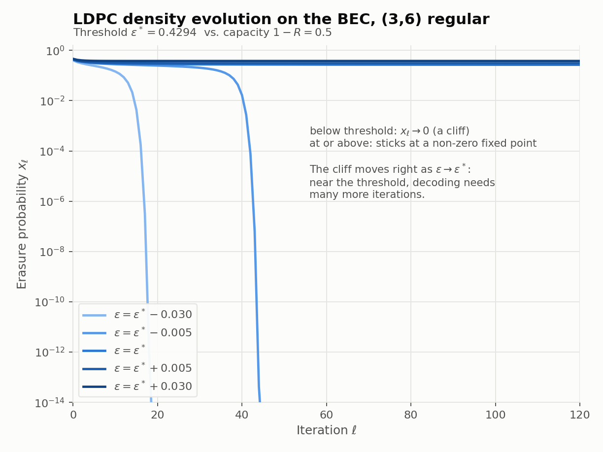

The figure shows the recursion actually run, and it repays a careful look. Below threshold, $x_\ell$ dawdles along a plateau and then plunges; this is the waterfall, seen from inside the math. At or above threshold, the trajectory flattens onto a fixed point and decoding fails no matter how long you iterate. And watch the cliff slide rightward as $\epsilon$ approaches $\epsilon^*$ from below: the closer to threshold you operate, the more iterations the plunge costs. That is not an artifact; it is the iteration-budget-versus-SNR trade-off that every practical decoder schedule fights, visible already in a three-line scalar recursion.

The Stability Condition

A fixed point at $x = 0$ is only useful if it attracts, and asking when it does yields the most-used practical result in RSU’s paper. Linearize the BEC recursion around zero. For small $x$, expand $\rho(1-x) = 1 - x\rho'(1) + O(x^2)$, so $1 - \rho(1-x) = x\rho'(1) + O(x^2)$; feed that through $\lambda$, using $\lambda(0) = 0$ (there are no degree-1 variable nodes), to get $\lambda(x\rho'(1) + O(x^2)) = \lambda'(0)\rho'(1)\,x + O(x^2)$. The recursion near zero is therefore $x_{\ell+1} = \epsilon\,\lambda'(0)\rho'(1)\, x_\ell + O(x_\ell^2)$, and the origin attracts precisely when the multiplier is below one. That is RSU’s Theorem 4, the stability condition on the BEC:

$\boxed{\;\lambda'(0)\,\rho'(1) \;<\; \frac{1}{\epsilon}.\;}$

For a general binary-input symmetric channel the message is a density rather than a number, so linearizing requires a scalar surrogate for “how much error remains.” The right surrogate is the Bhattacharyya functional $\mathfrak{B}(f) = \int f(x)\,e^{-x/2}\,dx$, chosen for two properties: it upper-bounds the error probability, and it is multiplicative under variable-node convolution, $\mathfrak{B}(f \circledast g) = \mathfrak{B}(f)\,\mathfrak{B}(g)$, because the integral is a two-sided Laplace transform evaluated at $-1/2$ and transforms turn convolutions into products. Running the same linearization with $\mathfrak{B}$ in place of $x$ gives the multiplier $\lambda'(0)\rho'(1)\mathfrak{B}(P_0)$, hence RSU’s Theorem 5: stability on a general channel requires $\lambda'(0)\rho'(1) < 1/\mathfrak{B}(P_0)$. Check it against the two channels you care about. On the BEC, the channel LLR is $+\infty$ with probability $1-\epsilon$ and $0$ with probability $\epsilon$, so $\mathfrak{B}(P_0) = (1-\epsilon)\cdot 0 + \epsilon \cdot 1 = \epsilon$, recovering the hand derivation exactly. On BI-AWGN, $P_0 = \mathcal{N}(\mu, 2\mu)$ with $\mu = 2/\sigma^2$, and the integral is the moment generating function at $-1/2$: $\mathfrak{B}(P_0) = \exp(-\mu/2 + 2\mu/8) = e^{-\mu/4} = e^{-1/(2\sigma^2)}$, giving the condition $\lambda'(0)\rho'(1) < e^{1/(2\sigma^2)}$.

Now read off what the two derivatives actually are. Every term of $\lambda'(x)$ except the first carries a factor $x^{i-2}$ that vanishes at zero, so $\lambda'(0) = \lambda_2$: the fraction of edges on degree-2 variable nodes. And $\rho'(1) = \sum_i \rho_i (i-1)$ is the average of $d_c - 1$ over edges. So the stability condition says, in engineering terms: the amount of degree-2 material you may use is capped, inversely, by the average check degree and by how bad the channel is.

Stop and notice what this is, because it is one of the best moments in the whole story. Gallager’s Theorem 2.5, from 1963, showed that codes built entirely from degree-2 variable nodes are hopeless: degree-2 nodes form chains, chains must close into cycles within $O(\log n)$ steps, and a closed cycle is a codeword of logarithmic weight. The stability condition is the same fact reborn in a different mathematical language. In 1963 the failure mode was “logarithmic minimum distance,” proved by counting tree tiers; in 2001 it is “the zero fixed point of density evolution is unstable,” proved by linearization. Same mechanism, same design rule, two formalisms 38 years apart. And the modern version sharpens the old one into a quantitative budget: degree-2 nodes are not forbidden, they are rationed, and RSU observe that capacity-approaching sequences on the BEC push $\lambda_2$ right up against the bound. The best codes spend the entire budget.

The Gaussian Approximation

Exact density evolution costs an FFT pipeline per iteration; a degree-distribution search needs millions of threshold evaluations; the product of those two facts is a practical bottleneck. Chung, Richardson and Urbanke supplied the workhorse shortcut: assume every message density is a symmetric Gaussian. Symmetry forces the consistency condition $s^2 = 2\mu$ you verified earlier, so a symmetric Gaussian is described by its mean alone, and the infinite-dimensional recursion collapses to a scalar one.

The variable-node half of the collapse is free. Means of independent summands add, so a degree-$i$ variable node outputs mean $\mu_v = \mu_0 + (i-1)\mu_c$ with $\mu_0 = 2/\sigma^2$ on BI-AWGN, and the variances add consistently too ($2\mu_0 + (i-1)\,2\mu_c = 2\mu_v$), so the Gaussian family is genuinely closed under this step. The check node is where the approximation lives. Take expectations of the tanh rule and define

$\phi(\mu) \;\triangleq\; 1 - \mathbb{E}\big[\tanh\tfrac{L}{2}\big], \qquad L \sim \mathcal{N}(\mu, 2\mu),$

a continuous, strictly decreasing function with $\phi(0) = 1$ and $\phi(\mu) \to 0$, so its inverse exists. Independence of the check inputs gives $1 - \phi(\mu_c) = \prod_j (1 - \phi(\mu_{v,j}))$, and this step is the approximation: the true check output is not Gaussian, and you re-Gaussianize it by matching this single moment. Averaging over both degree distributions yields the full irregular recursion,

$\mu_c^{(\ell)} \;=\; \phi^{-1}\!\left(1 - \sum_j \rho_j \Big[\,1 - \sum_i \lambda_i\, \phi\big(\mu_0 + (i-1)\,\mu_c^{(\ell-1)}\big)\Big]^{j-1}\right),$

started from $\mu_c^{(0)} = 0$. Divergence of $\mu_c$ to infinity means success; a finite fixed point means failure; bisection over $\sigma$ finds the threshold. The function $\phi$ has no closed form (tabulate it, or use the standard curve fits), the answers land within a few hundredths of a dB of exact DE, usually on the slightly optimistic side, and each threshold costs microseconds instead of seconds. That speed is what makes large-scale design search feasible.

Calibrate against the benchmark before trusting any implementation: the regular $(3,6)$ ensemble on BI-AWGN has exact-DE threshold $\sigma^* = 0.8809$, which is $E_b/N_0 = 1.11$ dB, about 0.9 dB from the Shannon limit of 0.187 dB for rate one half with binary input. If your Gaussian-approximation code lands near $\sigma^* \approx 0.88$, it works.

Optimization of Degree Distributions

Density evolution evaluates a degree profile; the remaining step is to search over profiles, and RSU’s crucial observation is that half the search is a linear program. Fix $\rho$ and the target channel. Maximizing the rate means maximizing $\int_0^1 \lambda = \sum_i \lambda_i / i$, which is linear in the unknowns $\lambda_i$. The constraints are linear too: normalization $\sum_i \lambda_i = 1$, non-negativity, stability $\lambda_2 < 1/(\rho'(1)\mathfrak{B}(P_0))$, and, the interesting one, convergence. Convergence constraints are linear because the DE map itself is linear in $\lambda$ for a fixed input density: the variable-node update is the $\lambda$-weighted sum $P_0 \circledast \sum_i \lambda_i R^{\circledast(i-1)}$, so “one iteration strictly reduces the error, starting from this checkpoint density” is one linear inequality per checkpoint. The working algorithm is a cutting-plane loop: solve the LP, verify with full density evolution, and if the recursion stalls at some intermediate error level, add that level as a new linear constraint and re-solve; then perturb $\rho$ by hill climbing (or run differential evolution over both polynomials) and repeat. The profiles that come out are strongly bimodal and tell the bootstrapping story of the opening section in numbers: a large mass of degree-2 and degree-3 variable nodes pressed hard against the stability bound, a small population of very high-degree nodes (degrees 15 to 30) to form the reliable core, and check degrees concentrated on one or two values.

The results, all at rate one half on BI-AWGN, are the headline of the paper and arguably of the decade:

Read the table bottom-up for the punchline. Chung and coauthors, pushing the same machinery with degree-thousands profiles, produced an ensemble whose threshold sits 0.0045 dB from the Shannon limit: for engineering purposes, capacity, reached by explicit design rather than existence proof. And RSU’s Figure 2 carries the sentence the field noticed most: their $n = 10^6$ irregular LDPC code, at 0.13 dB from capacity, “even surpasses the performance of turbo codes.” Eight years after the 1993 shock, the rediscovered 1963 code, armed with an exact theory the newcomer never had, retook the lead.

Practical Code Construction

Density evolution hands you an optimal $(\lambda, \rho)$, but a literally random graph with that profile is unusable: storing an arbitrary edge list for $n = 10^6$ and routing its wires through silicon is a non-starter. Real designs impose structure that preserves the degree profile while making the randomness cheap to describe:

The staircase row addresses a pitfall subtle enough to deserve its own sentence: a sparse $H$ does not give you cheap encoding. Decoding complexity lives in $H$, but encoding runs through the generator matrix, and Gaussian elimination on a sparse $H$ produces a dense $G$, making naive encoding $O(n^2)$. Two standard fixes exist. Richardson and Urbanke’s companion paper in the same 2001 journal issue shows how approximate lower-triangulation of $H$ yields $O(n)$ encoding plus a small dense correction; alternatively, design the staircase structure into the parity part of $H$ from the start, so parity bits fall out of a simple recursion. The second fix is why 5G looks the way it does: 5G NR specifies two QC protograph base graphs, BG1 (long blocks, rates 1/3 to 8/9) and BG2 (short blocks, rates 1/5 to 2/3), each with a staircase parity core, 51 lifting sizes for fine-grained length flexibility, and built-in punctured columns for rate matching. The decoding hardware story (why min-sum plus layered scheduling plus QC barrel shifters make LDPC the throughput king, and why interconnect rather than arithmetic is the real bottleneck) deserves its own treatment, and it gets one: the final page of this series takes the three code families into silicon together.

Trapping Sets and Error Floors

Honesty about limits, to close the technical story. Density evolution is an asymptotic, cycle-free theory, and there is a failure mode that lives exactly in its blind spot. A trapping set $(a, b)$ is a set of $a$ variable nodes whose induced subgraph has only $b$ odd-degree check nodes. If the channel corrupts roughly this set, the few unsatisfied checks cannot outvote the internally consistent (but wrong) mutual reinforcement of the $a$ variables, and the decoder locks into the wrong state; the stable-fixed-point variants, absorbing sets, are the worst offenders. These are finite-length cycle structures, precisely the objects the tree assumption erased, so density evolution says nothing about them. The practical consequence is the error floor: a code whose waterfall sits gorgeously close to capacity can flatten out at a BER of $10^{-7}$ and refuse to improve, and no threshold computation would ever have warned you. Threshold and floor are governed by different mathematics and are, to first order, independent properties; a better threshold does not mean a better code, and a serious design optimizes both, using girth- and trapping-set-aware construction (PEG, the ACE metric), post-processing decoders, or an outer algebraic cleanup code (DVB-S2 wraps its LDPC in BCH for exactly this reason). One related operational point: on a graph with cycles, belief propagation can converge to something that is not a codeword at all, so practical decoders cap the iteration count and use the syndrome test $H\hat{\mathbf{x}}^\mathsf{T} = \mathbf{0}$ as the stopping rule. That test is also a quiet luxury: an LDPC decoder knows when it has won, which turbo decoding never quite did.

Check Yourself

1. Why is analyzing transmission of the all-ones codeword legitimate, when a real transmitter sends arbitrary codewords?
2. Write the BEC density-evolution recursion and explain what each factor is doing.
3. Why does the check-node side of density evolution need the $\Gamma$ transform, while the variable-node side is an ordinary convolution?
4. What is the stability condition, what does $\lambda'(0)$ actually measure, and what 1963 result is the condition a descendant of?
5. Your new code has a threshold 0.08 dB from capacity but its BER curve flattens at $10^{-7}$. What is wrong, and can density evolution help you diagnose it?
6. In the trajectory figure, why does the cliff move to the right as $\epsilon$ approaches the threshold, and what does that cost in practice?

Where This Leaves Us

The arc that began with Gallager’s forgotten thesis is now complete. Sparse graphs make message passing cheap; local tree-likeness makes it nearly exact; concentration, the tree limit, and symmetry make the ensemble analyzable; the $\Gamma$ transform makes the analysis computable; and linear programming over degree distributions turns the analysis into a design tool that produced codes 0.0045 dB from Shannon’s limit and pushed past turbo. The same machinery also knows its own boundaries: everything asymptotic and cycle-free, nothing about the trapping sets and error floors where finite codes actually fail.

Step back, though, and turbo and LDPC share both a virtue and an unfinished question. Each gets its power by injecting randomness somewhere (turbo through the interleaver, LDPC through the random graph ensemble), and for neither is there a general proof of reaching capacity: LDPC thresholds can be driven as close to the limit as computation allows, but “0.0045 dB by numerical design” is an achievement, not a theorem, and Gallager himself proved that bounded check degrees keep capacity strictly out of reach. The next entry is about the code that closed this gap from an entirely different direction: polar codes, a deterministic, recursive construction with no randomness anywhere, and the first practical family provably achieving capacity.