Buses, Memory-Mapped Devices, Sensors & Actuators

Phase 3 took you inside the CPU: registers, caches, the memory hierarchy, interrupts. This phase moves outward to everything the CPU has to talk to across a shared wire, and then further outward still, to the physical world that sensors and actuators sit between. Wolf’s bus chapter explains how a processor addresses any memory-mapped device at all; Lee and Seshia’s sensors chapter explains how a physical quantity becomes a trustworthy digital number, or vice versa. Together they cover the complete path from a voltage on a wire to a CPU register and back out again to a spinning motor shaft.

The CPU Bus and the Four-Cycle Handshake

Underneath essentially every bus protocol sits the same small building block: the four-cycle handshake, an enq/ack raise-and-lower sequence that lets two devices agree “sender ready, receiver ready, data moved, both idle again” without needing a shared clock. It’s worth recognizing this shape wherever it recurs, because it isn’t unique to buses: RS-232’s start/stop bits and CSMA collision avoidance solve the same coordination problem at different layers of a system.

A concrete microprocessor bus bundles a handful of signals on top of that idea: a 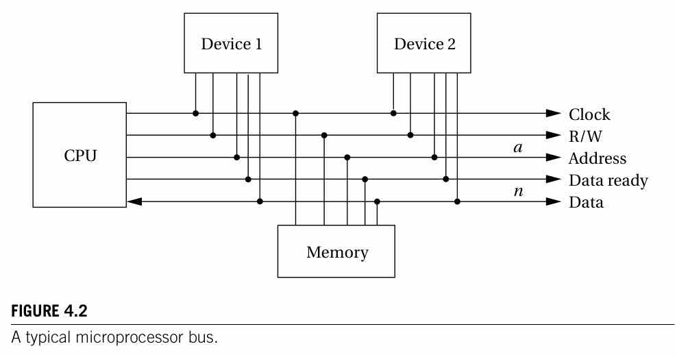clock, a R/W line, an address bus (a bits wide, unidirectional, since only the CPU decides where and what to access), a data bus (n bits wide, bidirectional), and a data ready line (often active low, for noise immunity). The standard notation for describing how these signals behave over time is the timing diagram: each signal is drawn as either a known value (0 or 1) or as stable/changing, with timing constraints (ordering requirements, and sometimes a minimum delay) marked between transitions.

Two features of the basic handshake are worth calling out because of what they buy you for free. Wait states let a slow device simply delay asserting data ready; this is exactly how cheap, slow memory coexists on the same bus as a fast CPU without any redesign of the protocol, since the handshake absorbs arbitrary device speed differences on its own. Burst transfers send one address followed by many sequential data values from consecutive memory locations, amortizing the per-transaction addressing and handshake overhead across N words, which is why burst mode matters so much for bulk transfers like video frames. Wolf makes both effects precise with a pair of bandwidth formulas. For a basic transfer, given bus clock period $P$, width $W$ bytes, $D$ cycles of actual data transfer, $O$ cycles of overhead, and $N$ bytes to move:

$$T = \left\lceil \frac{N}{W} \right\rceil (D + O), \qquad t = T \cdot P$$

and for a burst of $B$ transfers of $W$ bytes each, where the overhead $O$ is now paid once per burst rather than once per transfer:

$$T_{burst} = \left\lceil \frac{N}{BW} \right\rceil (B\cdot D + O)$$

DMA, Bus Mastership, and Multi-Bus Systems

The CPU isn’t the only device that can drive the bus. A DMA controller can become a temporary bus master, requesting control via its own bus request/bus grant handshake with the CPU and then performing reads and writes that are indistinguishable, from the memory or device’s point of view, from CPU-driven ones. While the transfer is underway, the CPU is free to keep doing useful work, provided that work doesn’t itself need the bus; the moment it does, it stalls until the DMA controller releases mastership. Real DMA controllers deliberately self-limit to short bursts (4, 8, or 16 words) specifically to bound how long the CPU can be locked out this way, trading some raw transfer efficiency for CPU responsiveness.

Bus design also scales by splitting into multiple buses joined by a bridge: a fast, expensive bus for high-speed devices, a slower, cheaper bus for everything else, and a bridge in between that acts as a slave on the fast side and a master on the slow side, translating both the data and the protocol timing. This is the same cost/performance segmentation idea as the memory hierarchy from Phase 3, applied to the bus instead of to storage: put expensive fast infrastructure only where it’s actually needed. ARM’s real AMBA bus family is the shipping example of this pattern: a high-performance, pipelined, burst-capable, multi-master AHB bus sits directly on the CPU, bridged out to a simpler, low-power APB bus that assumes a single master and serves ordinary peripherals.

Memory and I/O Interfacing

Even something as basic as how you lay out a memory chip’s bits is a real design decision. The aspect ratio of a memory (its depth-by-width trade-off for a fixed total size) can organize the same total bit count as very many narrow words or fewer wide ones, and the shape of your application’s data (RGB pixels, say) should drive which one is better.

DRAM introduces a subtler wrinkle: refresh is a scheduling problem, not just a circuit detail. A memory controller has to guarantee that every row gets refreshed within its spec window (on the order of milliseconds) while still serving ordinary reads and writes, so an access that happens to land during a refresh can stall. That’s a real, if usually small, source of timing variability, echoing the same predictability theme that came up around caches and the MMU in Phase 3.

Hanging an I/O device off the bus is a different problem from addressing memory, because a device typically needs far fewer distinct addresses. The standard technique is glueless interfacing: decode the device’s address with a comparator against a fixed high-order address range, and use a match to enable a transceiver, gating the R/W line so that a mismatch can never accidentally write the device. Wolf’s Example 4.1 works through exactly this pattern, and it generalizes cleanly: compare-then-enable-transceiver is the generic recipe for hanging almost any memory-mapped device off almost any bus it wasn’t natively designed for.

Two device-level quirks round out this section. A mechanical switch doesn’t settle cleanly when pressed, so a single press can look electrically like several; this switch bouncing is fixed either in hardware, with a one-shot timer circuit, or in software, by ignoring further transitions for a short window after the first one. It’s the identical phenomenon that Lee and Seshia’s sensors chapter flags for any mechanical switch used as a sensor. Scanned keyboards trade wiring complexity for an encoding limitation: a demultiplexer scans one row at a time, and the resulting row/column encoding can’t natively represent arbitrary simultaneous key presses, which is exactly why keyboard controllers need explicit n-key rollover logic to buffer or stack overlapping presses rather than just reading the raw array.

Finally, the ADC and DAC are the universal components at the analog/digital boundary. A DAC is comparatively simple: it just continuously converts whatever digital value happens to be latched. An ADC needs more: a start conversion clock or control input, plus, for converters whose conversion time depends on the value being sampled, a done signal, since unlike a DAC, an ADC’s conversion time isn’t fixed in advance.

System-Level Performance: Buses, Memory, and Software Together

It’s worth stepping back at this point to note that an embedded architecture is never purely a hardware exercise. Wolf is explicit that CPU choice, bus choice, memory, and I/O devices all sit on the hardware side of the ledger, but the CPU choice specifically “cannot be made without considering the software that will execute” on it. Architecture decisions run both ways.

That matters because system-level performance is not the same thing as CPU performance. The CPU only sets an upper bound; the bus and the memory each independently gate real throughput, and the bandwidth formulas above make that precise and computable rather than a vague warning. The real system-level speedup, in practice, comes from overlapping the two: splitting a computation into transfer and compute stages and letting the DMA controller run the next transfer while the CPU computes on the current data turns a sequential setup-wait-resume pattern into a pipelined one. It’s the same overlap idea as CPU instruction pipelining from Phase 3, just applied at the system/DMA level instead of inside a single CPU.

Sensors and Actuators: Modeling the Physical Boundary

A sensor or actuator is the literal boundary component between the analog, continuous, multidimensional physical world and the digital, quantized cyber world, and the real contribution of Lee and Seshia’s chapter is giving that boundary a precise, computable model instead of leaving it as “some noisy analog thing.”

The starting point is a linear model, $f(x(t)) = a\, x(t)$, where the proportionality constant $a$ is the device’s sensitivity. Real sensors and actuators are almost always better described by the affine model, which adds a bias term: $f(x(t)) = a\,x(t) + b$. Affine strictly contains linear (linear is just affine with $b = 0$), and a nonzero reading at zero input is the norm for real devices, not the exception.

That affine model only holds inside an operating range $(L, H)$; outside it, the output saturates at $L$ or $H$. The honest model of any real device is therefore piecewise affine: affine inside the range, flat and clamped outside it, and “is my signal still inside range” is a recurring, genuine design check rather than an edge case you can ignore.

Within that range, precision $p$ is the smallest difference in the physical quantity the sensor can still distinguish. For an ideal $n$-bit digital sensor over range $(L, H)$, precision and the related dynamic range $D$ (how many distinguishable steps fit inside the range) work out to:

$$p = \frac{H-L}{2^n}, \qquad D = \frac{H-L}{p} = 2^n, \qquad D_{dB} = 20\log_{10}(2^n) \approx 6.02\,n \text{ dB}$$

Dynamic range is naturally expressed in decibels because it spans orders of magnitude, and the rule of thumb worth keeping is that each extra bit buys roughly 6 dB, directly connecting “how many ADC bits do I need” to “what SNR do I need.”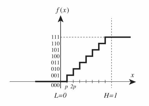

Noise gets the same formal treatment: a measured signal is the desired signal plus noise, $x'(t) = x(t) + n(t)$. The sharp observation here is that quantization itself is just a particular, deterministic form of additive noise, $n(t) = f(x(t)) - x(t)$, which is why quantization error and “real” sensor noise can both be analyzed with the same signal-to-noise machinery. SNR is the ratio of RMS signal to RMS noise:

$$N = \sqrt{\overline{n(t)^2}}, \qquad SNR_{dB} = 20\log_{10}\!\left(\frac{X}{N}\right)$$

and the earlier “6 dB per bit” rule turns out to literally be the SNR of ideal uniform quantization: two results that looked separate are really the same fact viewed twice.

Sampling introduces its own failure mode. Uniform sampling at interval $T$ (rate $1/T$ Hz) turns a continuous $x(t)$ into a discrete sequence, and distinct continuous signals can produce identical sample sequences, a phenomenon called aliasing, if you sample too slowly relative to their frequency content. The Nyquist-Shannon rule states this informally: sampling at rate $R$ uniquely captures signals whose fastest components fall below $R/2$. The standard fix is an anti-aliasing filter that removes high frequencies before sampling, since aliasing can’t be undone after the fact once it’s already happened.

A separate nonlinearity, distinct from saturation, is harmonic distortion: sensitivity itself varies with signal magnitude even within the nominal operating range. It’s modeled by adding power terms to the sensor’s transfer function, for example a second-harmonic term for a sinusoidal input $x(t) = a\sin(\omega_0 t)$:

$$f(x(t)) = b + a\,x(t) + d_2\,x(t)^2$$

which, via the identity $\sin^2\theta = \tfrac12 - \tfrac12\cos 2\theta$, produces energy at $2\omega_0$, the “second harmonic.” A pure input tone therefore picks up energy at multiples of its own frequency: audible in audio applications (human hearing is very sensitive to it) but often irrelevant elsewhere (human vision much less so), a good reminder that how much a given modeling nuance matters is application-dependent rather than a universal ranking.

The chapter’s fix for noise is signal conditioning: filter the noisy measurement $x' = x + n$ through an LTI system chosen to approximate $x$ while suppressing $n$. This works especially well when the signal and the noise occupy different frequency bands, as in the accelerometer example (a slow orientation change against fast vibration noise), where a lowpass filter separates them cleanly. Oversampling is the mirror-image trick applied on the input side: sample a coarse, even 1-bit, quantizer very fast and lowpass-filter the result to recover much better effective precision. Its actuator-side twin is the bang-bang controller, rapid 1-bit actuation averaged out by the plant’s own slow response, which is exactly the same principle that PWM exploits for actuators, discussed below.

Common Sensors, Actuators, and the DC Motor

An accelerometer measures proper acceleration, which by Einstein’s equivalence principle is inseparable from gravity; that’s why a stationary accelerometer reads tilt, since it’s really sensing the gravity vector’s projection onto its own axes. Integrating acceleration to get position accumulates drift, a bias error that grows as $t^2$ after double integration, which is exactly why inertial sensing alone is unreliable for absolute position over time and needs periodic external correction, such as GPS or any other known-good reset.

GPS itself is triangulation from four or more satellites’ precisely timestamped signals. The fourth satellite specifically exists to solve for the receiver’s own clock error, since a receiver-grade clock isn’t precise enough to trust on its own: three unknowns for position plus one for clock error means four equations are needed. An IMU performing dead-reckoning combines a gyroscope (orientation change) with an accelerometer (velocity change), integrating forward from a known starting point; it hits the same drift problem as plain accelerometer integration, and the same fix.

A simpler but no less real interfacing concern is just Ohm’s law. Given a supply voltage, a device’s voltage drop, and a current limit, you solve for the minimum series resistor, the everyday check behind something as ordinary as wiring up an LED:

$$V = IR, \qquad P = I^2R = VI$$

It’s the exact same “don’t exceed the GPIO current or voltage spec” concern that Wolf’s bus chapter raised in the abstract, now worked as a concrete numeric example.

That same cost logic explains why you generally switch, rather than linearly amplify, to drive a motor. A linear power amplifier that outputs a proportional voltage or current is expensive, bulky, and dissipates significant energy itself, while a simple on/off switch that tolerates high current is much cheaper to build. That’s why PWM, rather than a DAC feeding a linear amplifier, is the default way to control motor power, exploiting the same “the device’s response is slow relative to the switching frequency” principle that PWM uses for LEDs or heaters, but now applied to a system with real inertia and inductance to model.

The DC motor is the chapter’s best worked example of the actor-model machinery from Phase 1 applied to something concrete, because it’s a genuinely coupled electrical and mechanical system. Electrically, the coil behaves as a series R-L circuit plus a back-EMF term proportional to angular velocity, since the motor pushes back electrically simply by virtue of spinning inside a field:

$$v(t) = R\,i(t) + L\,\frac{di(t)}{dt} + k_b\,\omega(t) \qquad \text{(electrical, with back-EMF term } k_b\omega\text{)}$$

Mechanically, torque (proportional to current) drives angular acceleration via the rotational form of Newton’s second law, net of friction and any load torque:

$$I\,\dot\omega(t) = k_T\,i(t) - \eta\,\omega(t) - \tau(t) \qquad \text{(mechanical, Newton's 2nd law, rotational)}$$

where $v$ is applied voltage, $i$ is current, $\omega$ is angular velocity, $R$ and $L$ are the coil’s resistance and inductance, $k_b$ is the back-EMF constant, $k_T$ is the torque constant, $\eta$ is friction, $\tau$ is load torque, and $I$ is the moment of inertia. The two equations are coupled, not just chained: current affects torque affects velocity affects back-EMF affects current, a genuine feedback loop, and a nice real-circuit instance of the actor-model and feedback-control ideas from Phase 1.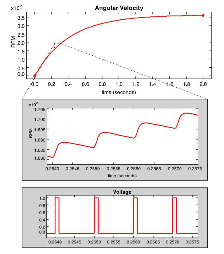

A rotary encoder converts shaft rotation into a pulse stream, and counting pulses per unit time gives angular velocity directly. It’s the sensor half of the standard closed-loop motor speed controller: PWM drives the motor following the feedback-control pattern from Phase 1, the encoder measures the actual result, and the error between target and measured speed feeds back into the duty cycle.

Where This Leaves Us

Wolf’s bus chapter and Lee and Seshia’s sensors chapter approach the same physical boundary from opposite directions. Wolf builds outward from the CPU: bus protocols, DMA, device address decoding, essentially “how does the processor talk to any memory-mapped thing.” LS builds inward from the physical world: sensor and actuator models, quantization, noise, sampling, essentially “how does a physical quantity become a trustworthy number, or vice versa.” Between them they cover the complete path from a physical phenomenon to a CPU register and back. The idea tying nearly every subsection together in both chapters is that every interface between two mismatched domains, whether that’s a fast bus and a slow device, analog and digital, continuous time and sampled time, or a desired signal buried in noise, needs an explicit protocol or model to bridge the mismatch cleanly: a four-cycle handshake, a wait state, an affine sensor model, an anti-aliasing filter. The DC motor is worth remembering specifically as the first fully worked feedback-control system since the helicopter example back in Phase 1, tying that actor-model math directly to a buildable circuit.

With the hardware side of the system now in view, from bus to boundary sensor, Phase 5 turns to the software that actually runs on top of it: program design, compilation, and optimization.