Software: Program Design, Compilation, Optimization

Phase 4 worked through how data actually moves between a processor and the outside world: buses, memory-mapped devices, sensors, actuators. This phase turns the lens back onto the software side of that same processor and asks a more basic question: once you’ve written a C program for an embedded target, what actually happens to it between the editor and the running chip, and how do you reason about the time, energy, and memory it will consume once it gets there? Wolf’s chapter on program design and analysis answers that in stages: reusable software patterns, a unifying graph model for any program, the full compiler-to-loader toolchain, a battery of optimization techniques, and finally the discipline of testing.

Building Blocks: State Machines, Buffers, and the CDFG

Two software patterns show up often enough in embedded code that they’re worth recognizing on sight. The first is the software state machine: an FSM’s behavior maps naturally onto a switch(state) block, where each case handles the guards and transitions for that state, and the fact that state stays the same “unless explicitly changed” gives you self-loops for free. This is literally the FSM notation from Phase 1 compiled down into C, and it’s worth recognizing as the same object every time it turns up in real code. It’s also the mirror image of something from Phase 3’s discussion of interrupt service routines and foreground processing: there, C code got lifted up into an FSM model for analysis; here, an FSM model gets lowered down into C for execution.

The second pattern is the distinction between circular buffers and queues. A circular buffer implements a fixed-size sliding window over streaming data (an FIR filter’s tap history is the classic case) without ever copying data: new samples simply overwrite the oldest ones via wraparound pointer arithmetic. A queue (an elastic buffer, backed by an array or a linked list) instead handles data arriving and departing at unpredictable rates. The distinction that actually matters in practice: a circular buffer assumes a fixed window size known in advance, DSP-style, while a queue assumes a variable, unpredictable backlog, event-style.

Underneath both of these, and underneath the rest of the chapter, sits one unifying model: the control/data flow graph (CDFG). A CDFG can describe any program, whether it’s written in C, assembly, or even hardware. Data flow graphs model straight-line basic blocks (single-entry, single-exit code with no conditionals), and decision nodes lay control on top of that. It’s the same “separate what varies in value from what varies in control” split that Phase 1 used to distinguish discrete from continuous dynamics, just applied here to program structure instead of physical dynamics.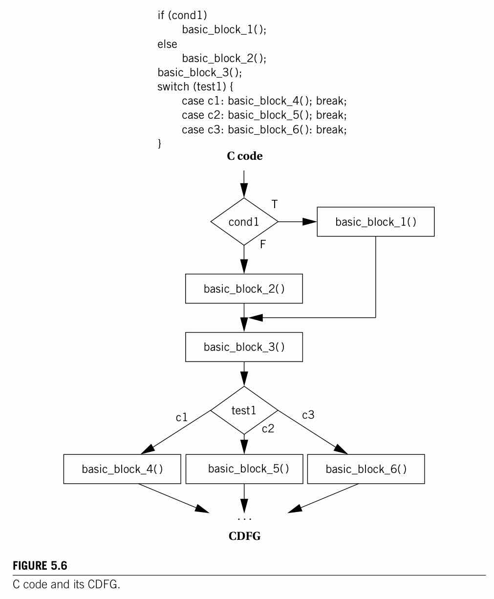

One requirement keeps a CDFG well-formed: single-assignment form, where each variable is assigned exactly once. Without it, multiple assignments to the same name would create a spurious cycle in the data flow graph. This isn’t just a drawing convenience: an acyclic DFG exposes the program’s actual data dependencies, which is exactly what a compiler needs in order to find safe instruction reorderings for pipeline and cache scheduling that the original sequential C code otherwise obscures. It’s worth treating the CDFG as more than an isolated modeling exercise, too: it’s the shared internal representation that compilers actually use to drive the optimizations covered later in this phase.

From Source to Silicon: Assembly, Linking, Loading, and Compilation

Getting from a C source file to a running program on an embedded target passes through a fixed pipeline: a compiler turns high-level code into assembly, an assembler turns that assembly into object code (resolving local labels along the way), a linker stitches multiple object files together and resolves external references into a single executable, and a loader places that executable into actual memory and starts it running. Understanding this chain matters for reasons beyond trivia, because embedded work routinely requires stepping outside it: hand-placing interrupt vectors, pinning code to a specific memory technology (EPROM versus DRAM), or controlling the exact address code gets loaded at.

The assembler itself works in two passes. Pass one walks the code purely to build a symbol table mapping labels to addresses, tracking a program location counter (PLC) that advances by each instruction’s encoded length as it goes. Pass two re-walks the code, substituting in the now-resolved addresses. It’s worth being precise about what the PLC is not: it makes exactly one linear pass through the code, unlike a runtime program counter, which revisits loop bodies repeatedly as the program actually executes.

A related choice is absolute versus relative (relocatable) addressing. Absolute addressing requires committing to a starting address (an ORG directive) before assembly even begins, which becomes impractical the moment a program is built from multiple independently-assembled files whose lengths aren’t yet known. Relocatable code instead defers address resolution to the linker, which is why relative addressing is the practical default for anything beyond a single-file program. That deferral is also exactly what the linker’s job consists of: matching every external reference (a use of a label defined elsewhere) in every object file against some other file’s entry point (where that label is actually defined), and reporting an error on anything left unresolved.

The compiler that produces the assembly in the first place follows its own standard pipeline: parsing and symbol-table construction and semantic analysis, then machine-independent optimization, then instruction selection paired with machine-dependent optimization, and finally emission of assembly code. Compilers stop at assembly rather than emitting raw binary specifically to avoid duplicating the assembler’s job.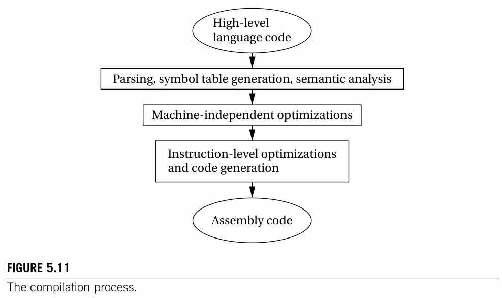

Wolf states the practical payoff of understanding this pipeline directly: knowing how a compiler generates code tells you when you can’t rely on it. For interrupt handling, exact data and instruction placement, and performance-critical sections, understanding the compiler’s translation choices is what lets you either write C that compiles the way you intend, or recognize the point at which you need to drop down to assembly instead.

Optimizing Loops

Most program optimization in this chapter comes down to loops, and three classic transformations recur throughout. Code motion hoists loop-invariant computation, a fixed loop-bound expression, say, out of the loop body so it’s computed once instead of on every iteration. Induction variable elimination replaces a recomputed index expression like i*M+j with an incrementally-updated running variable instead. Strength reduction replaces an expensive operation with a cheaper equivalent, turning a multiply-by-2 into a left shift, for instance. All three are really instances of one underlying idea: don’t recompute what a previous iteration has already established.

Cache behavior adds a subtler, nastier layer on top of these loop transforms. Array layout and traversal order directly determine how many conflict misses a loop nest generates, and the fix can be as cheap as shifting one array’s starting address by a few words to break a systematic block-aliasing pattern, which is exactly what Wolf’s Example 5.10 demonstrates. It’s a striking, non-obvious illustration of how a seemingly irrelevant memory-layout detail can end up dominating real performance, and it’s a direct callback to the direct-mapped-cache conflict-miss material from Phase 3. Below these loop-level transforms sit the compiler-internals stages of register allocation, scheduling, and instruction selection, which turn an optimized CDFG into real machine code. Wolf treats these mostly as classic-compilers vocabulary rather than as techniques you’d hand-apply yourself, and it’s worth carrying that vocabulary forward on the same basis.

Measuring and Predicting Performance

The organizing idea of the whole performance-analysis section is a single equation, and it’s worth committing to memory as a shape rather than as words:

$$\text{execution time} = \text{program path} \times \text{instruction timing}$$

The power of this equation is that its two factors can mostly be analyzed independently. First figure out which path through the CDFG actually executes: that’s a data-dependent question, answered by enumerating branch outcomes case by case or counting loop iterations. Then, separately, time that path’s specific instruction sequence.

It’s worth being explicit about why “count instructions and multiply by a per-instruction time” isn’t good enough on its own. Instructions don’t take uniform time (multi-cycle loads and floating-point operations especially), timing isn’t independent between adjacent instructions (pipeline forwarding effects couple them), and timing can depend on the actual operand values (a floating-point routine’s iteration count can be data-dependent). These are three independent sources of variability, stacking on top of whatever cache effects are already in play.

That variability is also why it’s worth distinguishing three separate performance measures rather than reporting a single number. Average-case performance needs a defined notion of “typical” input, which is often the hard part to pin down. Worst-case performance is the one that matters for meeting hard deadlines, and it’s the hardest to find the actual triggering input for. Best-case performance matters specifically for multirate real-time systems, a topic Phase 6 picks up directly.

Getting any of these numbers in practice means measuring, and the available methods range from cheap and imprecise to expensive and exhaustive: an on-chip timer bracketing a code region, a logic analyzer watching bus signals (limited by how deep its capture buffer is), and a cycle-accurate simulator, a full microarchitecture model including cache behavior, which runs slower than real hardware but exposes far more detail, and is the only practical way to get exhaustive timing data for something like flight-control-grade worst-case analysis. Wolf’s own SimpleScalar example illustrates a useful measurement trick along the way: control for fixed program overhead by scaling the iteration count N and comparing the normalized per-iteration cost, rather than trusting a single raw measurement.

Energy, Power, and Program Size

The single most useful number in this part of the chapter is that memory access, not computation, dominates a program’s energy cost: one measured figure puts a memory transfer at roughly 33 times the energy cost of an addition,

$$E_{\text{memory transfer}} \approx 33 \times E_{\text{addition}}$$

which reframes “optimize for energy” as “optimize memory access patterns and cache behavior” far more than “pick cheaper instructions.” Register access is the most efficient tier, cache comes next, and main memory trails a distant third.

Cache size interacts with energy in a way that’s genuinely non-monotonic. Too small a cache means frequent, expensive main-memory accesses dominate total energy; too large a cache means the cache itself, built from power-hungry SRAM, dominates energy even while its hit rate stays good. There’s a real middle optimum here, not a simple “bigger cache is always better” relationship, once energy rather than speed alone becomes the objective.

That leads to the best heuristic in the whole chapter, stated directly by Wolf: high performance equals low power. Most performance optimizations, fewer cache misses, fewer wasted cycles, reduce the total work a program does, which reduces its total energy consumption almost for free. That’s a notably different relationship than the predictability-versus-throughput tension that ran through Phase 2 and Phase 3: performance and energy are usually aligned goals here, not competing ones, in contrast to performance-versus-predictability, which usually does trade off.

Program size follows a similar “data first, instructions second” logic. Reducing data size (eliminating duplicate copies, sizing buffers to actual need rather than worst-imagined need, bit-packing flags) is usually higher-leverage than reducing instruction size, since code-size savings are capped by the real per-call overhead of a subroutine. Dense instruction sets, ARM’s Thumb and MIPS-16 among them, offer shorter encodings for a compatible instruction subset, and they’re a real, measured win: typically

$$\frac{\text{size}_{\text{dense}}}{\text{size}_{\text{standard}}} \approx 0.70 \text{ to } 0.80$$

of standard-encoding program size for the same functionality.

Testing for Correctness

Once performance, energy, and size are under control, the chapter turns to making sure the program is actually correct, and it frames testing as two complementary strategies rather than competing ones. Black-box testing exercises behavior only, without inspecting the code; clear-box (or white-box) testing generates test cases driven by the program’s internal structure. A thorough test plan uses both.

Underneath either strategy sit two prerequisites that are often the real bottleneck in practice, more so than any cleverness in choosing test cases: controllability, the ability to drive the program into the state you actually want to test, and observability, the ability to see the intermediate result you care about. Wolf’s Example 5.11, an FIR filter with a limiter, shows both failing at once: it’s hard to fill the buffer in a way that triggers clipping, and there’s no way to observe the pre-limit value without adding extra instrumentation.

Coverage criteria then formalize how thoroughly a test suite has exercised the code, and it’s worth being precise that statement coverage and branch coverage are not the same standard; they diverge specifically for unstructured code, raw assembly or goto-based state machines in C, where covering every statement doesn’t guarantee covering every branch direction. Basis paths, drawn from the graph-theoretic notion of a basis set and computed from the CDFG’s incidence matrix, formalize the smallest set of paths whose combinations cover every edge. The practical value is a principled minimum test-path count instead of guesswork, even though the underlying linear-algebra property technically only holds cleanly for undirected graphs, while CDFGs are directed. Since exhaustive path testing is provably infeasible for any program containing a loop or an unbounded input stream, the real skill this section teaches is choosing a defensible, finite subset of paths and branches to test; coverage criteria exist to make that choice principled rather than arbitrary.

Where This Leaves Us

This phase is where the hardware mechanics built up over Phases 2 through 4, pipelines, caches, buses, memory technology, cash out into concrete program-level engineering. The CDFG supplies a single model for any program’s control and data structure; the compiler-to-loader toolchain explains why embedded work routinely needs to step outside it; and three optimization axes (performance, captured by execution time as program path times instruction timing; energy, dominated by memory access at roughly 33 times the cost of an addition, with “high performance is low power” as the guiding heuristic; and size, dominated more by data than by instructions) give you the levers to actually act on that model. Testing closes the chapter as the complementary discipline for correctness once performance, energy, and size are under control. Nearly every technique here is really about predicting or shaping one of the two factors in the execution-time equation, or its energy and size analogues, which is exactly the skill Phases 2 through 4 were building toward. From here, the natural next question is what happens when a processor isn’t running one program at a time but many: Phase 6 picks that up directly, moving from “how long does this program take” to “which task gets to run next.”