Polar Codes: Capacity by Construction

Every capacity-approaching code this series has met so far runs on randomness. Turbo codes get theirs from an interleaver (a pseudo-random permutation that manufactures ensemble-like behavior inside a single code); LDPC codes get theirs from a randomly sampled sparse graph, analyzed through the ensemble it was drawn from. That was also Shannon’s own move in 1948: average over all codes, show the average is good, conclude a good code exists, and say nothing about how to find it. The series opener framed the sixty-year hunt that followed as the search for an explicit answer. In 2009, Erdal Arıkan delivered it: a deterministic construction, with no ensemble and no random draw anywhere, that provably achieves the symmetric capacity of any binary-input memoryless channel, with encoding and decoding both running in $O(N \log N)$. The mechanism is a single recursive idea called channel polarization, and this page builds it from one XOR gate up to the full theorem, then confronts the honest catch that kept polar codes out of practice for another few years.

Symmetric Capacity and the Bhattacharyya Parameter

Let $W: \mathcal{X} \to \mathcal{Y}$ be a binary-input discrete memoryless channel (B-DMC), $\mathcal{X} = \{0,1\}$. Arıkan’s analysis runs on two scalar parameters of $W$, and it matters that there are two, because they do different jobs.

The first is the symmetric capacity, the mutual information between input and output when the input is equiprobable:

$I(W) = \sum_{y\in\mathcal{Y}}\sum_{x\in\mathcal{X}} \tfrac{1}{2} W(y|x)\,\log_2 \frac{W(y|x)}{\tfrac12 W(y|0) + \tfrac12 W(y|1)} \;\in [0,1].$

The second is the Bhattacharyya parameter, a reliability measure:

$Z(W) = \sum_{y\in\mathcal{Y}} \sqrt{W(y|0)\,W(y|1)} \;\in [0,1].$

$Z(W)$ upper-bounds the maximum-likelihood error probability of a single use of $W$ to send one bit, so small $Z$ means a reliable channel. The two parameters track each other: $I(W) \approx 1$ exactly when $Z(W) \approx 0$ (a good channel), and $I(W) \approx 0$ exactly when $Z(W) \approx 1$ (a useless one). Arıkan’s Proposition 1 makes the coupling precise: $I(W) \ge \log_2 \frac{2}{1+Z(W)}$ and $I(W) \le \sqrt{1 - Z(W)^2}$.

Why carry both? Because $I$ measures rate and turns out to be the quantity that polarization conserves, which is what drives the main theorem; while $Z$ measures reliability, satisfies clean one-step recursions, and directly bounds error probability, which is what drives the performance theorem and the code construction. The proofs need each of them in its own role.

One special case is worth memorizing before anything else. For the binary erasure channel BEC($\epsilon$), which delivers the input bit with probability $1-\epsilon$ and an erasure symbol otherwise, both parameters are available in closed form: $I(W) = 1 - \epsilon$ and $Z(W) = \epsilon$. The BEC is the one channel where every quantity in this page can be computed exactly, which is why every worked example uses it.

Channel Combining and Splitting

Here is the entire invention at size two. Take two independent copies of $W$ and, before transmitting, couple their inputs with a single XOR:

$x_1 = u_1 \oplus u_2, \qquad x_2 = u_2.$

The combined two-bit channel is $W_2(y_1, y_2 \mid u_1, u_2) = W(y_1 \mid u_1 \oplus u_2)\, W(y_2 \mid u_2)$. Now split it back into two single-bit channels, defined so that they are decoded in order, $u_1$ first:

Read the definitions carefully, because the asymmetry between them is the whole trick. $W_2^{(1)}$, the channel seen by $u_1$, observes both outputs $y_1, y_2$ but must treat $u_2$ as unknown interference summed over; it is worse than a plain use of $W$. $W_2^{(2)}$, the channel seen by $u_2$, observes both outputs and receives $u_1$ as a known side input; it is better than $W$. Notice what that side input assumes: $W_2^{(2)}$ gets to act as if $u_1$ has already been decoded correctly. This “genie” assumption is written directly into the channel definition here, and successive cancellation decoding will later have to actually earn it, one bit at a time.

How much worse and how much better? Two exact statements answer this, and they are the load-bearing wall of the whole theory:

$\boxed{\,I(W_2^{(1)}) + I(W_2^{(2)}) = 2\,I(W)\,} \qquad \text{(conservation)}$ $\boxed{\,I(W_2^{(1)}) \;\le\; I(W) \;\le\; I(W_2^{(2)})\,} \qquad \text{(extremization)}$

Total capacity is preserved; it is merely redistributed. Nothing is created and nothing is destroyed: capacity is sorted, moved out of one channel and into the other. If you retain a single sentence from this page, make it that one, because everything that follows (the recursion, the polarization theorem, even the punchline of the martingale proof) is that sentence applied over and over.

Both statements have proofs short enough to keep in full. Conservation is nothing but the chain rule for mutual information. The map $(u_1,u_2) \mapsto (x_1,x_2)$ is a bijection (invert it: $u_2 = x_2$, $u_1 = x_1 \oplus x_2$), so if $U_1, U_2$ are i.i.d. uniform then so are $X_1, X_2$. Then

$I(W_2^{(1)}) + I(W_2^{(2)}) = I(U_1;Y_1Y_2) + I(U_2;Y_1Y_2 \mid U_1) = I(U_1U_2;Y_1Y_2) = I(X_1X_2;Y_1Y_2) = 2I(W),$

the last step because the two channel uses are independent. (The middle step uses the fact that $I(W_2^{(2)}) = I(U_2; Y_1Y_2U_1)$ equals the conditional term $I(U_2;Y_1Y_2 \mid U_1)$, since $U_2$ is independent of $U_1$.) $\blacksquare$

Extremization is the observation that adding observations cannot decrease mutual information:

$I(W_2^{(2)}) = I(U_2; Y_1Y_2U_1) \;\ge\; I(U_2;Y_2) = I(W),$

and conservation then forces $I(W_2^{(1)}) = 2I(W) - I(W_2^{(2)}) \le I(W)$. $\blacksquare$

The Bhattacharyya parameters transform just as cleanly:

$\boxed{\,Z(W_2^{(2)}) = Z(W)^2\,} \qquad \boxed{\,Z(W_2^{(1)}) \le 2Z(W) - Z(W)^2\,}$

with equality in the second relation if and only if $W$ is a BEC, a detail that will matter enormously when we try to construct codes for other channels. The first relation is an exact computation from the definition. The output alphabet of $W_2^{(2)}$ is the triple $(y_1, y_2, u_1)$, so

$Z(W_2^{(2)}) = \sum_{y_1,y_2,u_1} \sqrt{\tfrac12 W(y_1|u_1)W(y_2|0)\cdot \tfrac12 W(y_1|u_1\!\oplus\!1)W(y_2|1)}$ $= \tfrac12 \sum_{u_1}\Big[\sum_{y_1}\sqrt{W(y_1|u_1)W(y_1|u_1\!\oplus\!1)}\Big]\cdot \sum_{y_2}\sqrt{W(y_2|0)W(y_2|1)} = \tfrac12 \cdot 2Z(W)\cdot Z(W) = Z(W)^2,$

since the inner bracket equals $Z(W)$ for either value of $u_1$. $\blacksquare$

All of this abstraction becomes concrete in two lines on the erasure channel. For BEC($\epsilon$), where $Z = \epsilon$ is just the erasure probability: the first channel must recover $u_1 = x_1 \oplus x_2$, which requires both observations, so it is erased whenever either copy erases, with probability $1 - (1-\epsilon)^2 = 2\epsilon - \epsilon^2$. The second channel already knows $u_1$, so it can recover $u_2$ from either observation ($u_2 = y_2$ directly, or $u_2 = y_1 \oplus u_1$), and is erased only when both copies erase, with probability $\epsilon^2$. That two-line argument, “either erases” versus “both erase,” is the entire polarization mechanism made tangible, and it matches the two $Z$ formulas exactly.

Recursive Construction for Length N

One XOR moved capacity around a little. Arıkan’s next move is to do it again, recursively, on $N = 2^n$ copies of $W$: pair up channels and transform, then pair up the resulting synthetic channels and transform those, $n$ levels deep. Formally the length-$N$ combined channel is built from two length-$N/2$ ones,

$W_N(y_1^N \mid u_1^N) = W_{N/2}\!\left(y_1^{N/2} \,\middle|\, u_{1,\text{odd}}^N \oplus u_{1,\text{even}}^N\right)\cdot W_{N/2}\!\left(y_{N/2+1}^N \,\middle|\, u_{1,\text{even}}^N\right),$

and the split channels obey the one-step recursions you will use constantly:

The clean way to picture this is a binary tree of depth $n$. The root is $W$ itself; every node branches into a "$-$" child (the worse transform) and a "$+$" child (the better one). Each synthetic channel $W_N^{(i)}$ sits at a leaf, and the binary expansion of $i-1$ spells out the path that reaches it: index $i$ is a path through the polarization tree. A channel that took mostly "$+$" steps has been squared toward $Z \approx 0$ again and again and is nearly noiseless; one that took mostly "$-$" steps has been degraded toward $Z \approx 1$ and is nearly useless. The claim of the polarization theorem, proved below, is that as $n$ grows almost every leaf ends up at one extreme or the other, and the fraction landing at the good extreme is exactly $I(W)$.

If that claim holds, the code writes itself. Choose the $K$ most reliable synthetic channels as the information set $\mathcal{A}$ and send data on those; freeze the remaining $N - K$ inputs to values known in advance by both sides. The frozen bits are not overhead grudgingly accepted: they are the code. Freezing is precisely how the encoder avoids the bad synthetic channels, and the set $\mathcal{A}$ defines the code completely.

A Worked Example: Code Construction on the BEC

Nothing makes the mechanism believable like running it. Take $W =$ BEC($1/2$), so $Z(W) = 0.5$ and $I(W) = 0.5$, and recall that for the BEC both $Z$ recursions are exact equalities: $Z^- = 2Z - Z^2$ and $Z^+ = Z^2$. Iterating from $Z = 0.5$:

Check the conservation law at every level: the row sums are $0.5$, $1.0$, $2.0$, $4.0$, always $N\epsilon$, because for the BEC the parameter $Z$ is an erasure probability and erasure probability is conserved exactly. This is the arithmetic sanity check to run whenever you compute these by hand; if a row does not sum to $N\epsilon$, you made a slip.

Now sort the $N=8$ values: $0.004,\ 0.121,\ 0.191,\ 0.316,\ 0.684,\ 0.809,\ 0.879,\ 0.996$. They are visibly drifting toward the two extremes and away from the middle, though at $N=8$ the drift is still weak, a weakness we will return to with numbers attached. Push the same exact recursion to large $N$ and the drift becomes a cliff: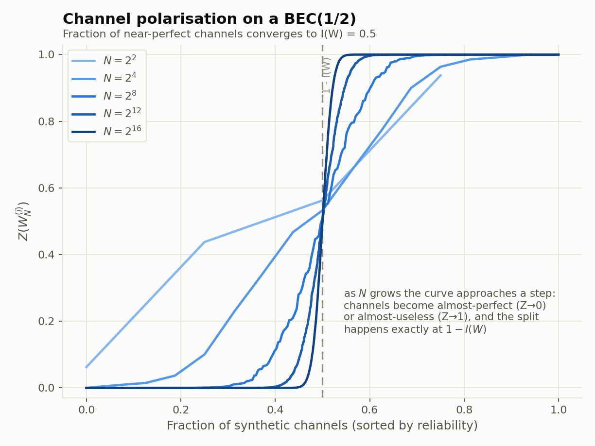

For a rate-$1/2$ code at $N = 8$ we need the $K = 4$ indices with the smallest $Z$:

$\mathcal{A} = \{4, 6, 7, 8\}, \qquad \mathcal{A}^c = \{1, 2, 3, 5\} \;\text{(frozen)}.$

Look at that set for a moment, because it kills a tempting misconception: $\mathcal{A}$ is not simply “the last $K$ indices.” Index 4 ($Z = 0.316$) beats index 5 ($Z = 0.684$), because index 4’s path through the tree ends in two "$+$" steps while index 5’s ends in two "$-$" steps. The reliability ordering is genuinely non-monotonic in the index, and it is channel-dependent besides.

How good is this code? Theorem 3 (stated properly below) bounds the block error probability of successive cancellation decoding by the sum of the information-set Bhattacharyya parameters:

$P_e \;\le\; \sum_{i\in\mathcal{A}} Z(W_N^{(i)}) = 0.316 + 0.191 + 0.121 + 0.004 = 0.633.$

Useless at $N = 8$, and the honesty is the point: polarization at small block lengths has barely begun, and this bound quantifies exactly the finite-length weakness Arıkan himself reports.

Finally, the encoder in matrix form. The recursive XOR structure works out to $\mathbf{x}_1^N = \mathbf{u}_1^N G_N$ with $G_N = B_N F^{\otimes n}$, built from Kronecker powers of the $2 \times 2$ kernel:

where $B_N$ is the bit-reversal permutation (for $N = 4$ it reorders rows to $1, 3, 2, 4$). The frozen positions $\mathbf{u}_{\mathcal{A}^c}$ are set to fixed values, conventionally zeros. Two convention warnings are worth flagging right here. First, $B_N$ only reorders; many modern treatments and the 5G standard drop it and work with the natural order $G_N = F^{\otimes n}$, giving the same code up to a permutation, so always check which convention a paper uses before comparing index sets. Second, the choice of frozen values is irrelevant only for symmetric channels (Arıkan proves this in his §VI); for asymmetric channels it genuinely matters, so “frozen bits are zero” is a convention, not a theorem.

Encoding and Successive-Cancellation Decoding

$F^{\otimes n}$ has the recursive butterfly structure of an FFT, and encoding inherits the FFT’s cost: $n = \log_2 N$ stages of $N/2$ XORs each, $\frac{N}{2}\log_2 N$ XOR operations total, computable fully in place with no matrix multiply and no memory beyond the codeword itself. Encoding a polar code is essentially free, a striking contrast with LDPC, where the sparse parity-check matrix gives no directly usable encoder and real systems need dedicated encoding structure.

Decoding is where the definitions of §2 come due. Successive cancellation (SC) decodes $u_1, u_2, \dots, u_N$ strictly in order. At step $i$:

Note the $\hat{u}_1^{i-1}$ in the conditioning: every decision assumes all previous decisions were correct. That is what “successive cancellation” means, it is exactly the decoder paying for the genie assumption baked into the definition of $W_2^{(2)}$, and it is also the algorithm’s central flaw, because a single early error corrupts everything downstream. Hold that thought for the finale.

Computationally, everything reduces to two update functions applied on a binary tree of depth $\log_2 N$. Given two log-likelihood ratios $a$ and $b$ arriving from the channel side:

$f(a,b) = 2\,\mathrm{artanh}\!\left(\tanh\tfrac{a}{2}\tanh\tfrac{b}{2}\right) \approx \mathrm{sign}(a)\,\mathrm{sign}(b)\,\min(|a|,|b|)$

combines two LLRs whose underlying bits are XOR-coupled, and

$g(a,b,\hat{u}_s) = b + (1 - 2\hat{u}_s)\,a$

combines them once the coupling bit $\hat{u}_s$ (the partial sum) is known. Stop and recognize $f$. It is identical to the check-node update of LDPC belief propagation: the same tanh rule, the same min-sum approximation, for the same reason (a check node also computes the LLR of an XOR of bits). And $g$ is the variable-node update with a sign flip. Polar SC decoding and LDPC message passing are built from the same two primitives; they differ only in the graph the primitives run on and the schedule that fires them. This series has been telling a story of three apparently unrelated code families, and at this moment the story collapses into one: everyone is doing sum and tanh-product updates on a graph, and the families differ in where the graph comes from.

Both functions drop straight out of the $N = 2$ splitting definitions, and the derivation is short enough to keep. Write the channel LLRs $L_1 = \ln\frac{W(y_1|0)}{W(y_1|1)}$ and $L_2 = \ln\frac{W(y_2|0)}{W(y_2|1)}$. For $f$, expand $W_2^{(1)}$ by summing over $u_2$: under $u_1 = 0$ the transmitted pair is $(u_2, u_2)$ and under $u_1 = 1$ it is $(1 \oplus u_2, u_2)$, so

$W_2^{(1)}(y_1,y_2 \mid 0) = \tfrac12\big[W(y_1|0)W(y_2|0) + W(y_1|1)W(y_2|1)\big],$ $W_2^{(1)}(y_1,y_2 \mid 1) = \tfrac12\big[W(y_1|1)W(y_2|0) + W(y_1|0)W(y_2|1)\big].$

Divide numerator and denominator by $W(y_1|1)W(y_2|1)$ to get the LLR of the first synthetic channel:

$L^{(1)} = \ln\frac{e^{L_1}e^{L_2} + 1}{e^{L_1} + e^{L_2}}.$

To see this equals the tanh form, set $t = \tanh\frac{L_1}{2}\tanh\frac{L_2}{2} = \frac{(e^{L_1}-1)(e^{L_2}-1)}{(e^{L_1}+1)(e^{L_2}+1)}$ and use $2\,\mathrm{artanh}(t) = \ln\frac{1+t}{1-t}$. Over the common denominator, $1 + t$ has numerator $(e^{L_1}+1)(e^{L_2}+1) + (e^{L_1}-1)(e^{L_2}-1) = 2e^{L_1+L_2} + 2$, while $1 - t$ has numerator $2e^{L_1} + 2e^{L_2}$, so $\frac{1+t}{1-t} = \frac{e^{L_1+L_2}+1}{e^{L_1}+e^{L_2}}$, matching $L^{(1)}$ exactly. $\blacksquare$

For $g$, the second synthetic channel has $u_1$ available as side information:

and both cases at once read $L^{(2)} = L_2 + (1 - 2u_1)L_1$. $\blacksquare$

The asymmetry of the transform is now visible as algebra. $f$ attenuates: $|f(a,b)| \le \min(|a|,|b|)$, so the "$-$" channel’s evidence is weaker than either input. $g$ adds: it accumulates both LLRs, so the "$+$" channel’s evidence is stronger. That is polarization, restated in two lines about absolute values. One practical note falls out of the min-sum approximation, which keeps only the dominant exponentials for large $|L_1|, |L_2|$: unlike LDPC min-sum, polar decoders usually apply it without a correction scaling factor, because SC makes a hard decision immediately and never iterates, so there is no feedback loop for min-sum’s over-confidence to amplify.

The full decoder is a depth-$\log_2 N$ tree recursion: descend left applying $f$, wait for the left subtree’s decoded bits, descend right applying $g$ with those bits as partial sums, then combine and pass upward. Condensed:

# α: LLR vector of length m = 2^(n-d) at a depth-d node
# β: returned hard-decision vector (partial sums) of the same length

def decode(node, α):
    if node.is_leaf:                       # m == 1, one bit
        if node.frozen: return [0]
        return [0] if α[0] >= 0 else [1]   # threshold the LLR

    m = len(α) // 2
    αl = [ f(α[i], α[i+m])         for i in range(m) ]
    βl = decode(node.left, αl)
    αr = [ g(α[i], α[i+m], βl[i])  for i in range(m) ]   # needs βl!
    βr = decode(node.right, αr)
    return [βl[i] ^ βr[i] for i in range(m)] + βr        # combine upward

û = decode(root, [channel_LLR(y[i]) for i in range(N)])

Three details of this recursion are each a classic source of bugs, so they earn explicit notice. First, the line computing αr cannot run until βl has returned: the right subtree’s input depends on the left subtree’s output. Second, the returned β vectors are partial sums, the re-encoded values at that tree level, not information bits; the information bits are read off at the leaves as they are decided. Third, the combine step [βl ^ βr] + βr is precisely the encoder’s butterfly run in reverse: SC decoding re-encodes as it goes, which is also why the partial sums exist at all.

Complexity is $O(N \log N)$ time, and with a small observation, $O(N)$ memory: a naive implementation stores an LLR array at every node for $O(N \log N)$ space, but at any instant only one array per level is live, and level $d$ holds $2^{n-d}$ values, so $\sum_{d=0}^{n} 2^{n-d} = 2N - 1$ suffices.

The first of those three details deserves its own paragraph, because it is not a bug hazard but an architectural sentence. The $g$ step for any right subtree cannot start until its left sibling has fully decoded, and this dependency chain runs the entire length of the code: SC decoding is inherently serial, bit after bit after bit. Where LDPC belief propagation updates every node in the graph simultaneously and soaks up parallel hardware, SC decoding fundamentally resists it. This serial dependency will haunt the hardware story when the series reaches it.

The Polarization Theorem

Everything so far assumed the channels actually do polarize. Arıkan’s Theorem 1 states it: for any B-DMC $W$ and any $\delta \in (0,1)$, as $N = 2^n \to \infty$,

In words: the fraction of near-perfect synthetic channels converges to exactly the capacity, the fraction of near-useless ones to exactly one minus the capacity, and nothing survives in the middle.

The proof is the elegant core of the paper, and it fits in five steps. Define a random walk down the polarization tree: at each level, step to the "$-$" child or the "$+$" child with probability $1/2$ each, and let $I_n$ be the symmetric capacity of the synthetic channel you are standing on after $n$ steps. Choosing a uniformly random leaf this way makes statements about the walk statements about the fraction of leaves, which is what the theorem needs.

1. $\{I_n\}$ is a martingale: by conservation, $\mathbb{E}[I_{n+1} \mid I_n] = \tfrac12(I^- + I^+) = I_n$, and it is bounded in $[0,1]$.
2. Bounded martingales converge almost surely, so $I_n \to I_\infty$.
3. Convergence forces the two branches to stop separating: $|I^+ - I^-| \to 0$ along the walk. But the extremization inequality says the branches genuinely separate unless the channel is already extremal, with $I \in \{0,1\}$.
4. Therefore $I_\infty \in \{0,1\}$ almost surely: the limit is a Bernoulli random variable.
5. The martingale property pins down its mean: $\mathbb{E}[I_\infty] = I_0 = I(W)$, so $\Pr[I_\infty = 1] = I(W)$. $\blacksquare$

The last line is the punchline of the entire subject, and it is worth saying slowly. The fraction of perfect channels equals the capacity because capacity was conserved at every single step. Conservation makes the capacity process a martingale; the martingale property survives to the limit; and so whatever mass ends up at $I = 1$ must, on average, equal what you started with. The sorting metaphor was not decoration: the proof is literally an accounting identity. And notice what the proof does not use: no distance spectrum, no ensemble average, no union bound over codewords. It is barely a page. A companion argument runs the same walk on $Z_n$, which is a supermartingale ($Z^+ = Z^2 \le Z$ and $Z^- \le 2Z - Z^2$) also converging to $\{0,1\}$, and that version is what actually feeds the error bound.

Finite-Length Performance

The performance statement is Arıkan’s Theorem 3: for the polar code defined by information set $\mathcal{A}$,

$\boxed{\,P_e(N, K, \mathcal{A}) \;\le\; \sum_{i\in\mathcal{A}} Z(W_N^{(i)})\,},$

and for any fixed rate $R < I(W)$, choosing $\mathcal{A}$ as the $NR$ best indices gives $P_e = O(N^{-1/4})$, independently of the rate, with $O(N \log N)$ encoding and decoding. This is the headline of the paper and the answer to the series question: an explicit, deterministic code family that provably achieves the symmetric capacity of any B-DMC with quasi-linear complexity. Shannon’s 1948 promise, made constructive, sixty-one years later.

But look at that convergence rate. $N^{-1/4}$ is slow: pushing $P_e$ to $10^{-6}$ this way would need $N$ on the order of $10^{24}$. Arıkan does not hide it; his §V-D numerical example concludes, in his own words, that “the example also shows that the rate of polarization is too slow to make near-capacity polar coding under SC decoding feasible in practice.” His Figure 7 is the quantitative form of that sentence: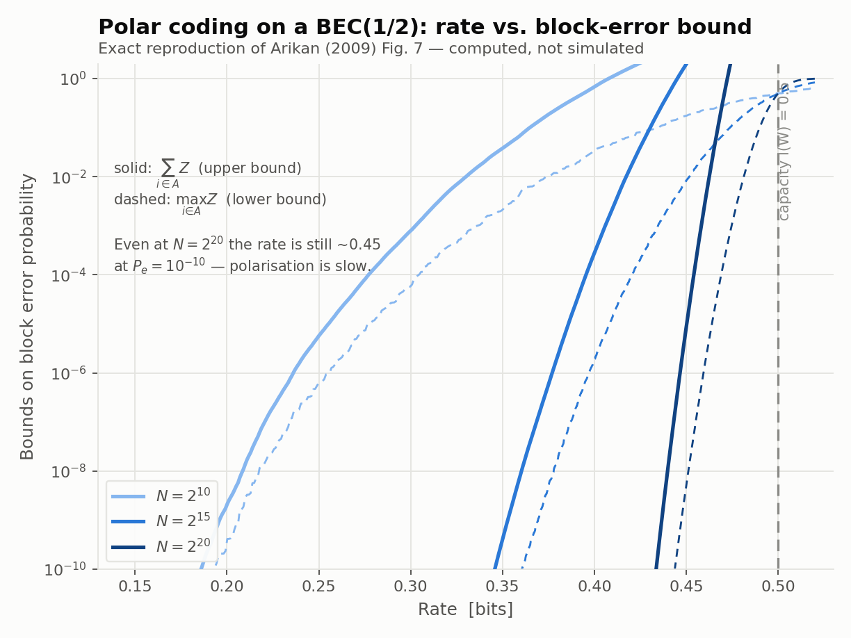

Even at $N = 2^{20} \approx 10^6$, holding the error bound below $10^{-10}$ costs you rate: about $0.45$ against a capacity of $0.5$. Arıkan and Telatar later tightened the asymptotics dramatically, to $P_e \approx 2^{-N^\beta}$ for any $\beta < 1/2$, but the finite-length gap is real and it sets up this page’s ending: capacity-achieving does not mean best at practical lengths. At the block lengths real systems use, a plain SC-decoded polar code loses to a well-designed LDPC code. Asymptotic optimality and finite-length competitiveness are different properties, and in 2009 polar codes had only the first.

Code Construction and Comparison with Reed-Muller Codes

One more practical matter hides inside “choose the $K$ indices with smallest $Z$”: computing those $Z$ values. Arıkan’s §IX is refreshingly honest that this is hard in general, because the exact $Z^-$ recursion holds only for the BEC; for any other channel the synthetic channels’ output alphabets grow exponentially and no efficient exact algorithm is known. The methods that emerged form a ladder:

Two consequences follow. First, a polar code is channel-specific: the information set depends on the design SNR, and a set designed for one operating point loses performance at another. One code per design SNR is an awkward property for a standard, and the 5G row of the table is precisely the engineering compromise that resolves it: a single tabulated nested ordering that is good enough across operating points. Second, polarization itself helps construction: as $N$ grows, most $Z$ values cluster so close to $0$ or $1$ that even a coarse estimate classifies them correctly.

Arıkan closes his paper with a comparison that carries a design lesson bigger than polar codes. Reed-Muller codes have exactly the same matrix structure $G_N = F^{\otimes n}$; they differ only in choosing $\mathcal{A}$ by row Hamming weight instead of by $Z$. His §X proves that the RM rule is asymptotically unreliable under SC decoding. The reason is that the RM rule is channel-blind: it maximizes minimum distance, which is the right criterion for maximum-likelihood decoding, but SC is not ML. SC is a sequential procedure whose error probability is governed by $\sum_{i\in\mathcal{A}} Z(W_N^{(i)})$, a channel-dependent reliability sum that the row-weight rule ignores entirely. (Amusingly, at $N = 8$ on BEC($1/2$) the two rules happen to select the same set $\{4,6,7,8\}$; the agreement is a small-$N$ coincidence, and the RM choice degrades as $N$ grows.) The general lesson: the right design criterion depends on the decoder you will actually use. RM optimizes for ML, polar optimizes for SC, and this is the same lesson the turbo story taught when the effective free distance and the error coefficient, not $d_{\text{free}}$, turned out to govern iteratively decoded performance. Codes are not good or bad in the abstract; they are good or bad for a decoder.

Check Yourself

1. What quantity is conserved by the polarization transform, and what exactly does that conservation buy in the proof of Theorem 1?
2. Why does $W_2^{(2)}$ end up better than $W$, while $W_2^{(1)}$ ends up worse?
3. State the two $Z$ recursions. Which one is exact only for the BEC, and why does that matter in practice?
4. For BEC($0.2$), compute all four $Z(W_4^{(i)})$, verify the conservation check, and choose the information set for rate $1/2$.
5. Reed-Muller codes use the same $F^{\otimes n}$ structure. Why does choosing $\mathcal{A}$ by row weight fail under SC decoding when it is the right rule under ML decoding?
6. Why is SC decoding hard to parallelize, at the level of the tree recursion?

Where This Leaves Us

Arıkan’s 2009 paper closed the question this series opened: a fully explicit, deterministic code with $O(N\log N)$ encoding and decoding and a one-page martingale proof that it achieves capacity, no random ensemble anywhere. Along the way it quietly unified the field, since the SC decoder’s $f$ and $g$ are exactly the check-node and variable-node primitives of LDPC message passing, running on a different graph under a different schedule. But the same paper is candid about its two weaknesses: polarization is slow, so at practical block lengths the plain SC-decoded polar code loses to LDPC; and SC decoding is greedy and irrevocable, so one early wrong decision corrupts everything after it, with no mechanism for repair. A provably capacity-achieving code that ships worse performance than its theoretically ungrounded rivals: that is where 2009 left polar codes, and it took until Tal and Vardy to change it. Their fix, keeping a list of candidate decoding paths and letting a CRC pick the winner, not only rescued the decoder but exposed and then repaired a deeper weakness of the code itself, and it carried polar codes all the way into the 5G standard. That story, list decoding, the CRC trick, and the hardware endgame, is the finale.