List Decoding and the Road to 5G

The previous entry ended on an uncomfortable cliffhanger. Polar codes are the only family in this series with a proof of capacity achievement, complete with $O(N \log N)$ encoding and decoding, and yet at any block length you could actually build, plain successive-cancellation polar codes lose to LDPC. A theorem that wins in the limit and a code that loses on the bench: something had to give. This finale tells the story of what gave, in three acts. First, Tal and Vardy’s list decoder, which closed the gap and in doing so uncovered a deeper problem than the one it set out to solve. Second, the hardware reality check, where all the “this will matter later” threads scattered through this series (turbo’s serial trellis sweeps, LDPC’s parallel graph, polar’s sequential decision chain) finally get cashed in as silicon. Third, the verdict: a survey of 110 decoder chips that refuses to crown a winner, and a 5G standard that agreed with it by splitting the crown in two.

Successive-Cancellation List Decoding

Start with an honest diagnosis of what is wrong with successive cancellation. SC is greedy and irrevocable: it decides $\hat u_1$, then $\hat u_2$ given $\hat u_1$, and so on, and no decision is ever revisited. Decide $\hat u_3$ wrongly and every later decision is conditioned on a corrupted history; the error propagates down the chain and nothing downstream can repair it. What makes this genuinely painful is that the fatal decision is usually a near miss. At the moment of the mistake, the correct value was only slightly less likely than the wrong one, and a decoder with even a little hindsight would have recovered.

Before fixing it, separate two deficits that are easy to blur and that the whole rest of this page turns on. The decoder deficit is the gap between SC and maximum-likelihood decoding of the same polar code: SC is simply not extracting all the information the code offers. The code deficit is the gap between the polar code’s own ML performance and what a great code of that length could do, and it exists because polar codes have mediocre minimum distance at short and moderate lengths. Tal and Vardy set out to attack the first deficit, discovered that closing it exposed the second, and then fixed that one too. Keep the distinction in hand; it is the plot of act one.

Their algorithm, successive-cancellation list decoding (SCL), replaces the single greedy path with up to $L$ concurrent candidate paths through the decision tree. At each frozen bit, every path is extended with the known frozen value; no branching happens. At each information bit, every path forks into two children, one taking $\hat u_i = 0$ and one taking $\hat u_i = 1$, giving up to $2L$ paths, which are immediately pruned back to the $L$ most plausible. At the end, the decoder outputs the best surviving path. The near-miss error that kills SC is now survivable: the correct continuation may drop to second place at the bad bit, but second place stays on the list, and later evidence can promote it back.

Ranking the paths requires a running score, and the form used in practice is an LLR-domain path metric that is numerically stable and addition-only. Writing $L_i^{(\ell)}$ for the decision LLR that path $\ell$ computes for bit $i$ (using the same $f$ and $g$ recursions as plain SC), the metric updates as

with lower being better. The hardware-friendly approximation makes its meaning transparent: if the chosen bit $\hat u_i$ agrees with the sign of $L_i^{(\ell)}$, the metric is unchanged; if it contradicts the sign, the metric pays a penalty of $|L_i^{(\ell)}|$. A path’s score is simply its accumulated penalty for arguing with the channel, and cheap paths are paths that have contradicted the evidence rarely and only when the evidence was timid. Note that frozen bits still charge the toll: if the LLR at a frozen position points the wrong way, every path pays $|L_i|$ there, which is exactly how a corrupted history makes itself visible in the metric.

Efficient Implementation of List Decoding

The obvious implementation of forking is a disaster. Each path carries the full internal state of an SC decoder (the LLR arrays and partial-sum bit arrays at every level of the recursion, $O(N)$ numbers in total), and copying that state at every fork, for each of the roughly $N$ information bits, costs $O(L N^2)$ overall. For $N$ in the thousands that is unusable, and this is where Tal and Vardy’s paper earns its place: the algorithmic idea is simple, but the data structure that makes it affordable is the real contribution.

The insight is that two paths that just forked are identical except for one bit, so copying their entire state duplicates almost all of it for nothing. Instead, paths share array segments until one of them writes: a fork merely increments reference counts on the shared arrays, and the actual copy is deferred to the moment a path first needs to modify an array it does not exclusively own. This is reference-counted copy-on-write, the same pattern as persistent data structures in functional programming, applied per level of the decoding tree. The essential structure of the two key steps fits in a few lines:

# fork/prune at an information bit
for each active path ℓ:
    score PM[ℓ] + penalty(L, 0)  and  PM[ℓ] + penalty(L, 1)
keep the best L of the 2L candidates        # a sort, on the critical path
kill paths with no surviving continuation   # frees their slots first
clone paths whose 0- and 1-children both
survived: bump refcounts, copy nothing      # O(log N), not O(N)

# copy-on-write accessor
getLLR(depth, ℓ):
    if path ℓ is the sole owner of its array at this depth:
        return it (safe to write in place)
    else:
        split off a private copy now, and only now

Why does this land on $O(L N \log N)$? Count the copy work for one path through a full decode, level by level. A node at depth $d$ of the decoding tree is visited $2^d$ times, and each visit can trigger at most one copy of an array of length $2^{n-d}$ (with $N = 2^n$). So depth $d$ contributes at most $2^d \cdot 2^{n-d} = N$ units of copying, and summing over the $n+1$ depths gives $(n+1)N = O(N \log N)$ per path, hence $O(L N \log N)$ in total, with $O(LN)$ memory. The lazy copy is the entire difference between this and the naive $O(L N^2)$: list decoding costs only $L$ times plain SC, which is what made SCL a practical proposition rather than a thought experiment.

One line of that pseudocode deserves a flag planted next to it, because it will grow into a major plot point in act two: keep the best $L$ of the $2L$ candidates. That selection is a sorting operation, it happens at every information bit, and it is serial and comparison-heavy, sitting squarely on the decoder’s critical path. In software it is a rounding error; in hardware it will turn out to dominate.

CRC-Aided List Decoding

So how well does the list do? Tal and Vardy’s Figure 5, at block lengths 2048 and 8192 and rate 1/2, shows performance improving monotonically with $L$, but with unmistakable diminishing returns, and by $L = 32$ the curve sits essentially on the ML bound: the performance an optimal decoder of the same code would achieve.

That claim needs a way of measuring the ML bound, since running true ML decoding at these lengths is exactly the impossibility this series opened with, and their method is quietly clever. Whenever the $L = 32$ decoder fails, check whether the codeword it produced was more likely than the transmitted one, that is, whether $W(\mathbf{y} \mid \hat{\mathbf{c}}) > W(\mathbf{y} \mid \mathbf{c})$. If so, a true ML decoder, which by definition picks the most likely codeword, would have failed on this noise realization too. The frequency of that event is therefore a lower bound on the ML error probability, measured without ever running an ML decoder. The SCL curve at $L = 32$ sits on that bound.

Pause on what this means, because it is the pivotal realization of the paper. At $L = 32$ the decoder is, for practical purposes, optimal: the decoder deficit is gone. Growing the list further is pointless, not because lists stop helping in some vague asymptotic sense, but because there is provably nothing left for a better decoder to recover. The bottleneck has moved from the decoder to the code. Polar codes at these lengths have mediocre minimum distance, and SCL at $L=32$ has slammed into the code’s own ML wall. (This also disposes of a tempting misconception: “bigger list is always better” is false past this point; beyond $L \approx 32$ you are spending exponentially growing effort to approximate a ceiling you have already reached.)

Fixing a code deficit ought to require a new code. Tal and Vardy found something much cheaper, by looking at how the $L = 32$ decoder fails: on a large fraction of failures, the correct codeword was still in the final list, just not in first place. The decoder had done its job of carrying the truth to the finish line; it merely lacked a way to recognize it there. What they needed was a genie to point at the right list entry, and a genie is easy to build out of standard parts: a CRC. Of the $k$ unfrozen bits, use the first $k - r$ for information and the last $r$ for a CRC of those information bits. At the end of decoding, discard every path whose CRC fails, then output the most likely survivor (if none passes, output the most likely path anyway, and know that an error has occurred). The rate cost is tiny; the performance gain is dramatic.

It is worth being precise about why this works, because the lazy reading (“the CRC detects errors”) misses the point entirely. The CRC here is functioning as an outer code: the concatenation of CRC and polar code is a new code whose minimum distance is far better than the polar code’s alone, because the low-weight polar codewords that caused the ML wall almost never satisfy the CRC constraint and so stop being codewords of the concatenated system. What makes the combination click is that SCL is precisely the decoder able to exploit an outer code, because it delivers $L$ candidates rather than one; a CRC bolted onto plain SC would have nothing to select among. CRC-aided SCL is a coding gain, not a detection feature, and the gain is large enough to flip the league table: CA-SCL polar beats LDPC at short block lengths, by around a dB. This is CA-SCL, and it is what 5G would eventually standardize.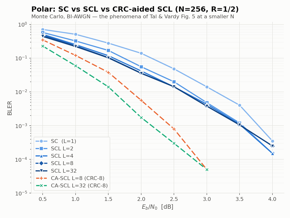

The figure replays the whole act at $N = 256$, in three ideas: keep the runners-up, notice that the wall is the code’s, repair the code from outside.

Hardware Implementation Considerations

Act two changes the judging criteria. Everything so far has been measured in dB; the race to 5G was run in Gb/s, mm² of silicon, and pJ per bit, and under those metrics the three families’ structural properties, flagged repeatedly across this series, finally come due.

Start with turbo, and recall from the turbo analysis that its decoder runs BCJR over a trellis, twice per iteration. Per the Shao survey, turbo loses the throughput race for three compounding reasons, all of them serialization. First, BCJR itself is serial: the $\alpha$ recursion sweeps forward through the block and the $\beta$ recursion sweeps backward, and the backward sweep cannot begin until the block ends; sliding-window variants help but cap the available parallelism. Second, the two constituent decoders are serial with respect to each other: DEC 2 consumes DEC 1’s extrinsic output, so they take turns rather than working at once. Third, when you try to recover parallelism by splitting the block across multiple BCJR engines, the interleaver fights back: several engines read and write the same memory banks through the permutation $\pi$, and the resulting contention stalls the pipeline. LTE’s answer was the QPP (quadratic permutation polynomial) interleaver, which is provably contention-free, a nice example of a hardware constraint reaching back and redesigning a code component. And on top of all three, iterations multiply latency, and 5G’s latency budget is unforgiving. Yet the same survey is emphatic about where turbo still wins: turbo decoders showed the best raw error-correction performance of the three families and the highest flexibility, with natural support for arbitrary block lengths and, especially, for very low code rates, where both LDPC and polar efficiency degrade while turbo’s stays flat.

LDPC is turbo’s structural opposite, and the properties Gallager built in from the start are exactly the ones silicon rewards. One belief-propagation iteration costs $O(E)$, where $E$ is the edge count of the Tanner graph, linear in block length, and, crucially, every node update is independent: all check nodes can fire simultaneously, then all variable nodes. That is massive parallelism as a property of the algorithm, not of any particular implementation. The engineering refinements stack neatly on top: layered scheduling roughly halves the iteration count by letting updated messages propagate within a sweep; min-sum reduces the check-node update to comparisons and additions, no multipliers and no lookup tables; and quasi-cyclic (QC) structure turns the “random” permutation into a barrel shifter, a trivially routable piece of hardware. The honest limit is elsewhere: for fully parallel decoders the bottleneck is interconnect, not arithmetic. A flooded graph at $n = 2048$ means thousands of messages crossing the die every iteration, and routing congestion, not the compute, sets the chip area. The survey makes the point explicitly: implementation complexity is computational complexity plus interconnect complexity plus flexibility, and QC structure is precisely what tames the second term. The one soft spot, noted above, is that LDPC efficiency degrades at low code rates.

And polar? Its congenital defect is that SC is a sequential decision chain: bit $i$ needs $\hat u_1^{i-1}$, so the dependency chain spans the whole block, the mirror image of LDPC’s all-at-once updates. The hardware literature surveyed by Giard and colleagues is essentially a ladder of increasingly aggressive attacks on that chain. The first rung is the observation that plain SC visits all $2N - 1$ nodes of the decoding tree, most of them pointlessly, because whole subtrees have trivial structure:

A Fast-SSC decoder ends up looking like a small processor: memories for soft and hard values, and a controller driven by an instruction list that encodes the specific polar code, so changing the code means loading a new instruction list. That is where polar’s claimed flexibility lives in practice. Unrolled decoders sit at the other extreme: hundreds of Gb/s reported, but the code is hard-wired and the pipeline registers consume serious area, with a tunable compromise (accept a new frame every $I > 1$ cycles, cutting register cost roughly by $I$).

There is also a road around the chain rather than up it: polar codes can be decoded by belief propagation on their encoding factor graph, the same $f$/$g$ primitives run iteratively and in parallel, LDPC-style. BP-on-polar buys parallelism, low latency, and a genuinely soft output (SC is not soft-in soft-out, which matters for iterative detection and turbo equalization); it pays with worse error correction than SCL and many iterations. It is polar’s admission that when raw parallelism is the requirement, the LDPC way is the way.

Which leaves SCL, the decoder that actually delivers polar’s coding gain, and here the flag planted in act one comes down. In SCL hardware the dominant cost is not the $f$/$g$ arithmetic but path-metric sorting: selecting the best $L$ of $2L$ candidates at every information bit is a serial, comparison-heavy operation on the critical path, and it dominates both area and latency. Specialized sorting networks and approximate pruning schemes that skip unlikely forks help at the margins, but the shape of the trade is fixed: high throughput forces small $L$, and small $L$ throws away the coding gain that justified SCL in the first place. That tension is polar’s central hardware problem, and it frames everything in act three.

Comparison and Standardization in 5G NR

The Shao survey compares 110 ASIC implementations across the three families, and its head-to-head table, trimmed here to the rows that carry the story, reads like a character sheet for everything this series has covered:

Read down any column and you find no clean sweep; read across any row and you find a different name in bold. The survey’s own bottom line is refreshingly blunt: turbo has the best error correction and the most flexibility but serial BCJR caps its throughput and efficiency; LDPC reaches high throughput and high area and energy efficiency and is the workhorse for high-rate data; polar gives a dB or more of coding gain at short lengths but achieving high throughput forces small lists that squander it. No code dominates, and the survey explicitly declines to name a winner.

The 5G NR standardization process reached the same conclusion, and its reasoning chains are worth reciting in full because every link is something this series derived. The data channel (eMBB) went to LDPC. Data blocks are long, hundreds to thousands of bits, which is exactly where polar’s short-block advantage vanishes. The throughput requirement is extreme, multi-Gb/s, which LDPC’s node-parallel decoder meets and serial BCJR cannot. And data traffic needs HARQ with incremental redundancy, retransmissions that send additional parity rather than repeating the block; LDPC supports this naturally through rate-compatible puncturing of a base graph, while HARQ for polar codes was still an unsolved problem at the time of the survey. The standard’s concrete answer is two quasi-cyclic, layered-decodable base graphs, BG1 for long high-rate blocks and BG2 for short low-rate ones.

The control channels went to polar. Control blocks are short, tens to a few hundred bits, exactly polar’s sweet spot, where CA-SCL’s advantage over LDPC is real and about a dB. The reliability requirement is severe while the throughput requirement is mild, so a decent list size is affordable. Polar has essentially no error floor, which matters enormously for control signalling, where an undetected error is catastrophic rather than merely inconvenient. And the clincher is almost an accounting trick: control messages carry a CRC anyway for error detection, so the outer code that CA-SCL needs is already sitting in the frame, and CRC-aided list decoding is very nearly free.

And turbo was dropped, which is the part worth saying carefully. It was not dropped for being a bad code; by the survey’s own measurements it has the best raw error-correction performance of the three families and would still be the first choice at very low code rates. It was dropped because at 5G’s throughput, latency, and efficiency targets, every one of its three serializations loses to LDPC, and being the best code is not the job. Being the best decoder in silicon at the operating point is the job. If this series has a single engineering moral, that sentence is it.

One frontier note before closing: Arıkan’s own answer to polar’s distance problem, PAC codes, which replace the CRC with a convolutional pre-transformation and approach the finite-length bounds at short lengths, is where this story currently continues.

Check Yourself

1. SCL at $L = 32$ sits provably on the ML bound, so no better decoder for the polar code exists. Why does CRC-aided SCL then do better, and why is calling the CRC “error detection” a misreading?
2. How did Tal and Vardy measure the ML bound without ever running an ML decoder?
3. What dominates the area and latency of an SCL decoder in hardware, and what unpleasant trade does that force at high throughput?
4. Turbo codes had the best raw error-correction performance in the Shao survey. Give the three serialization reasons they were nevertheless dropped from 5G.
5. Why is a fully parallel LDPC decoder’s bottleneck interconnect rather than arithmetic, and which structural trick tames it?
6. Reconstruct both 5G reasoning chains: why LDPC for the data channel, and why polar for control?

Where This Leaves Us

Step back far enough and the whole series is one argument. The 1948 question asked how to get random-like performance from a structure you can actually decode, and the three families answered it with three different sources of randomness: turbo drew it from a long pseudo-random interleaver stitched between two weak codes, LDPC drew it from the random sparse graph itself, and polar used none at all, manufacturing its performance from a deterministic recursion and proving it with a martingale instead of an ensemble average. Underneath the three answers sits one computational substrate: every decoder in this series is message passing on a factor graph, LLRs combined and filtered by the same handful of primitives, whether flooded across a Tanner graph under density evolution’s asymptotic guarantee, exchanged as extrinsic information between two trellises, or marched in fixed order through a butterfly network and, in the end, multiplied into a list. And the resolution of the whole story is that Shannon’s challenge has a plural answer: the best code turned out to depend on the operating point (block length, rate, throughput, latency, floor tolerance), so 5G ships two of the three families side by side and retired the third for reasons that have nothing to do with coding gain. That is the end of the 5G story, but this series has one page left in it: a coda on sparse regression codes, which never came near a cellular standard but answer the opening question by a route unrelated to any of turbo, LDPC, or polar, worth reading precisely because it is so different. If you want to keep pulling the thread beyond that, the natural next reads are Arıkan’s PAC codes, where the polar story is still being written, and the 3GPP NR specification itself, where everything in these seven pages is frozen into tables.