A Fourth Answer: Sparse Regression Codes and AMP

The previous entry closed the series’ main narrative: turbo, LDPC, and polar codes, three distinct sources of structured randomness, evaluated against one another on their own merits. This page does not reopen that discussion. It is an epilogue, covering a fourth code family built on principles unrelated to any of the three preceding ones, that nonetheless answers the opening question of this series: how does one obtain random-like performance from a structure that is actually decodable? Sparse regression codes answer it in a way that is arguably closer to Shannon’s original 1948 argument than turbo, LDPC, or polar codes ever were. Where those three families obtained tractability by imposing structure on the code itself (a sparse graph, two short trellises, a deterministic recursive transform), sparse regression codes take the opposite approach: the code is left essentially unstructured, as in Shannon’s original construction, and all of the engineering effort is placed in the decoder instead. This final page examines why that approach works.

Overview and Motivation

The construction can be summarized before introducing any of its supporting machinery. A codebook is built the way a statistician, rather than an algebraist, would: a large dense matrix $A$ with independent Gaussian entries, partitioned into $L$ sections of $M$ columns each. A codeword is formed by selecting one column from every section and summing the selected columns, each scaled by a prescribed amount of power. The transmitted message is simply which column was selected in each section, so the code is an instance of a classical statistical estimation problem, sparse linear regression: recovering a sparse coefficient vector $\beta$ from noisy linear measurements $y = A\beta + w$. A literal decoding rule would require a search over $M^L$ candidates, as computationally intractable as the $2^k$ candidates left by Shannon’s own random code in the series opener. This intractability is resolved by an approximate message passing (AMP) iteration, which exploits the Gaussianity of $A$ to reduce the search to a short sequence of closed-form steps: a softmax denoiser applied section by section, corrected at every step by a single scalar Onsager term that keeps the recursion asymptotically well behaved. The resulting code, established in 2017, is provably capacity-achieving on the AWGN channel with $O(N \log N)$ encoding and decoding complexity, reaching the same destination as turbo, LDPC, and polar codes by an entirely different route.

Every other family in this series approached the decoding problem the same way: impose sparse structure, a sparse parity-check graph, two short trellises linked by an interleaver, a sparse recursive transform, so that local, low-complexity message passing could substitute for a global maximum-likelihood search. Sparse regression codes reverse this approach. The design matrix $A$ is close to maximally unstructured: dense, with independent Gaussian entries and no sparsity to exploit. This is deliberate, and it is what places SPARCs closest, among the families in this series, to Shannon’s original 1948 argument. Shannon’s proof used a random codebook of size $2^{nR}$ and established that a random draw is good with high probability, without providing a tractable decoder. A SPARC is a structured random codebook: the section structure, exactly one nonzero entry per section, is what makes efficient decoding possible, while the dense Gaussian matrix is what allows the capacity proof to proceed using the tools of classical statistical estimation (least squares, and later AMP) rather than graph combinatorics. It is Shannon’s construction, constrained just enough to be decodable, rather than a different construction entirely.

This history closely parallels the opening page of this series. Gallager proved his codes good by an ensemble argument in 1963 but left behind a decoder that no contemporary hardware could run; an efficient decoder did not arrive for thirty years. SPARCs followed the same arc on a considerably shorter timeline.

	The code was proven good…	…but the decoder was
Gallager 1963 (LDPC)	ensemble argument, maximum-likelihood decoding	computationally unthinkable in 1963
Barron and Joseph 2010 (SPARC)	least-squares decoding, exponentially small error for any $R < C$	least squares over a combinatorial constraint set, no efficient algorithm known
Joseph, Barron, and Cho (efficient successive decoders, early 2010s)	efficient decoding	error probability decays only like $n/\log n$, and flat power allocation caps the achievable rate at $R_0 < C$, strictly below capacity
Rush, Greig, and Venkataramanan 2017 (AMP)	efficient and capacity-achieving for every $R < C$	$O(N\log N)$ with a Hadamard design matrix

The third row is central to the argument of this page. The earlier efficient decoders, including adaptive successive decoding and Cho and Barron’s soft-decision decoder, function correctly, but under flat power allocation they provably cannot exceed a threshold rate $R_0 = \tfrac12 \tfrac{P}{P+\sigma^2}$, strictly below capacity $C = \tfrac12\log_2(1+P/\sigma^2)$. No improvement to the decoder alone removes this limitation, since the cap is imposed by how power is distributed across sections rather than by the algorithm that reads them. AMP is the first decoder that is simultaneously computationally efficient and loses nothing up to capacity, and it achieves this only because the power allocation was redesigned alongside the decoder. Rush, Greig, and Venkataramanan’s paper effectively presents two contributions under a single title: a new decoder, and the power allocation schedule that the decoder requires in order to be effective.

Code Construction and Power Allocation

The design matrix is $A \in \mathbb{R}^{n \times ML}$, with entries drawn independently as $A_{ij} \sim \mathcal{N}(0, 1/n)$, organized as $L$ sections of $M$ columns each. The message vector $\beta \in \mathbb{R}^{ML}$ has exactly one nonzero entry per section, of magnitude $\sqrt{nP_\ell}$ in section $\ell$, where $\sum_{\ell=1}^L P_\ell = P$ is the total power budget. The codeword is $x = A\beta_0$, the sum of $L$ columns of $A$, one per section, each scaled by that section’s power. Transmitting $x$ over the AWGN channel gives the receiver $y = A\beta_0 + w$ with $w \sim \mathcal{N}(0, \sigma^2 I_n)$. Encoding is straightforward: the input bit stream is split into $L$ chunks of $\log_2 M$ bits, and chunk $\ell$, read as an integer, selects which of section $\ell$‘s $M$ columns is active.

The rate equation follows from a codeword count. There are $M^L$ possible messages, so $M^L = 2^{nR}$, equivalently $L \log_2 M = nR$. Choosing $M = L^{\mathsf{a}}$ for a fixed constant $\mathsf{a} > 0$ gives $\mathsf{a}\, L \log_2 L = nR$, which forces $L = \Theta(n / \log n)$: both $L$ and $M$ grow with block length, but only slightly sub-linearly, so the dictionary size $n \times ML$ grows polynomially rather than exponentially in $n$. It is instructive to consider the two limiting cases. Setting $L = 1$, $M = 2^{nR}$ recovers Shannon’s original exponential-size random codebook exactly. Setting $L = n$ with a small constant $M$ makes the construction resemble the generator matrix of a conventional linear code. A SPARC is deliberately positioned between these extremes, what Barron and Joseph term a “moderate size dictionary”: structured enough for efficient decoding, unstructured enough for the dense-matrix machinery of AMP to apply.

The remaining design choice, the power allocation $\{P_\ell\}$, is not a secondary detail. It determines how the fixed power budget is distributed across sections and is as consequential for a SPARC as the degree distribution $(\lambda, \rho)$ is for an irregular LDPC code: two codes with identical $n$, $L$, and $M$ can achieve substantially different rates depending solely on this choice. The simplest option is flat allocation, $P_\ell = P/L$ for every section, which is the allocation identified above as fundamentally limiting: under efficient decoding it caps the rate at $R_0 < C$ regardless of decoder quality. The allocation for which AMP’s capacity theorem is proved instead decays exponentially, $P_\ell \propto 2^{-2C\ell/L}$, so the earliest sections carry disproportionately more power than later ones.

The intuition behind this choice underlies much of the rest of the page. Early, well-powered sections decode first and reliably. Once decoded, they are no longer unknowns: the decoder subtracts their contribution, which lowers the effective noise experienced by the harder, later sections. Each successfully decoded section makes the next section’s decoding task easier, a bootstrapping process that decodes the codeword section by section, from front to back. This mechanism is the SPARC analogue of the principle by which high-degree variable nodes converge first and assist the rest of the graph in irregular LDPC ensembles, transplanted from a degree distribution over a sparse graph to a power schedule over a dense one.

The AMP Decoding Algorithm

Initialize $\beta^0 = 0 \in \mathbb{R}^N$ (with $N = ML$) and $z^{-1} = 0$. For $t = 0, 1, 2, \dots$, AMP alternates a residual update and a denoising update:

$z^{t} \;=\; y - A\beta^{t} \;+\; \frac{z^{t-1}}{\tau_{t-1}^2}\left(P - \frac{\|\beta^{t}\|^2}{n}\right)$

$\beta^{t+1}_i \;=\; \eta^t_i\!\left(\beta^t + A^{\!\top} z^t\right), \qquad i = 1,\dots,N$

with $\tau_0^2 = \sigma^2 + P$ and, for $t \ge 0$, $\tau_{t+1}^2 = \sigma^2 + P(1 - x_{t+1})$, where $x_{t+1}$ is a Gaussian expectation computed offline, prior to decoding (discussed in the next section). The denoiser $\eta^t$ acts section by section: for index $i$ in section $\ell$, given a test-statistic vector $s$, it looks at all $M$ entries of $s$ within that section and computes

$\eta^t_i(s) \;=\; \sqrt{nP_\ell}\;\frac{e^{\,s_i\sqrt{nP_\ell}/\tau_t^2}}{\displaystyle\sum_{j\in\mathrm{sec}(\ell)} e^{\,s_j\sqrt{nP_\ell}/\tau_t^2}}$

which is a softmax over the $M$ candidates in the section, with inverse temperature $\sqrt{nP_\ell}/\tau_t^2$: sharply peaked when one entry of $s$ clearly dominates its section, and diffuse when the section remains ambiguous.

Each term in the recursion has a clear functional role. $A^\top z^t$ correlates the current residual against every column of $A$, acting as a matched filter: columns aligned with the (as yet undiscovered) true signal produce a large response, while unaligned columns remain near zero. Adding this to the current estimate gives $s^t = \beta^t + A^\top z^t$, the test statistic, which combines fresh matched-filter evidence with the decoder’s current belief. The denoiser $\eta^t$ then converts this test statistic into the next estimate, section by section. The remaining term in the residual update, $\dfrac{z^{t-1}}{\tau_{t-1}^2}\left(P - \dfrac{\|\beta^t\|^2}{n}\right)$, is the Onsager term: a single scalar multiplying the previous residual, added into the new one. Although it resembles a minor correction, it is essential to the algorithm’s validity, as the next section establishes.

The origin of this recursion clarifies why it takes exactly this form. Rush, Greig, and Venkataramanan derive the residual and denoising updates as a first-order Taylor approximation to a min-sum-style message-passing algorithm on the factor graph of $y = A\beta + w$: rows act as check-like factor nodes and columns as variable nodes, the same graphical vocabulary used by Gallager’s Tanner graph, except that here the graph is complete rather than sparse, since every observation depends on every coordinate of $\beta$. The one-nonzero-per-section constraint prevents the recursion from reducing to ordinary compressed-sensing AMP, in which each coordinate is denoised independently: here, every entry within a section is coupled to every other entry in that section, so the outgoing message from one variable depends on the incoming messages from its entire section rather than on itself alone. This coupling is why the denoiser takes the form of a joint softmax over a section rather than $M$ independent scalar shrinkage rules, and it is SPARC’s counterpart to the requirement that a parity check exclude the very bit it is informing.

The Onsager Correction Term

The validity of the entire recursion rests on a claim about the distribution of the test statistic. Asymptotically,

$s^t \;\overset{d}{\approx}\; \beta + \bar\tau_t Z, \qquad Z \sim \mathcal{N}(0, I_N) \text{ independent of } \beta$

that is, $s^t$ behaves as the true message plus clean, independent Gaussian noise, despite having been constructed from $A$, the same matrix used to construct every earlier $\beta^t$. Without the Onsager correction, $s^t$ would carry a self-interaction bias: because $\beta^t$ was fit using $A$, the quantity $A^\top z^t$ correlates with $\beta^t$ through their shared dependence on the same matrix, so the residual “noise” in $s^t$ would be neither clean nor Gaussian. The state-evolution analysis in the following section depends on this Gaussian approximation holding exactly, not merely approximately, and the Onsager term is what makes it hold.

This mechanism is directly comparable to two earlier appearances of the same principle in this series, and the resemblance is structural rather than superficial:

Code	What gets excluded	So that…
LDPC belief propagation (check to variable)	the receiving variable’s own previous message	no self-reinforcing loop around a short cycle
Turbo decoding (extrinsic LLR)	the channel value and a priori value at that specific bit	the second decoder does not just parrot the first decoder’s opinion back at it
SPARC AMP (Onsager term)	the first-order self-interaction of $\beta^t$ with the matched-filter output	$s^t$ stays asymptotically Gaussian and independent of $\beta$

This is the same exclusion principle appearing a third time, here in a continuous rather than combinatorial setting. LDPC and turbo decoding both remove self-information because their underlying graphs contain short cycles that would otherwise allow a decoder’s own earlier output to feed back into itself, amplified rather than corrected. AMP’s graph has no sparsity to exploit: every observation depends on every coordinate, so every pair of variables is effectively one hop apart. The Onsager correction is what remains of the exclusion principle once the graph is maximally dense: there is no longer a specific neighbor’s message to exclude, so the recursion instead subtracts a single scalar quantity, calibrated to cancel exactly the bias that density would otherwise introduce.

This dependence introduces an implementation pitfall worth noting, since it is the SPARC analogue of a trap this series has already encountered. The residual-update equation explicitly requires $z^{t-1}$ and $\tau_{t-1}^2$, the previous step’s residual and constant, in the correction added to the new residual. Substituting the current step’s $z$ and $\tau$ instead causes $s^t$ to silently lose its asymptotic Gaussianity; the state-evolution analysis in the next section, and empirically the decoder’s performance, then breaks. This is a one-line indexing error with a disproportionate effect, comparable in spirit to SCL’s “kill before clone” ordering requirement: a subtle sequencing constraint, embedded in a single equation, on which the entire analysis silently depends.

Optimality of the Section-Wise Denoiser

The softmax form of $\eta^t$ may appear to be a heuristic chosen for convenience, but it is in fact the provably optimal estimator. Given the Gaussian approximation established above, $s^t = \beta + \tau_t Z$, the minimum mean-squared-error estimate of $\beta$ given $s^t$ is the conditional expectation $\mathbb{E}[\beta \mid s^t]$, which can be derived for one entry $i$ in section $\ell$ directly from Bayes’ rule, treating the $M$ candidates in the section as equally likely a priori:

$\beta_i^{t+1}(s) = \mathbb{E}[\beta_i \mid s^t = s] = \sqrt{nP_\ell}\;\frac{f(\{s_j\}_{j\in\mathrm{sec}(\ell)}\mid \beta_i=\sqrt{nP_\ell})}{\sum_{k\in\mathrm{sec}(\ell)} f(\{s_j\}_{j\in\mathrm{sec}(\ell)}\mid \beta_k=\sqrt{nP_\ell})}$

Since $Z$ is i.i.d. Gaussian, each conditional density is proportional to $\exp(s_k\sqrt{nP_\ell}/\tau_t^2)$, up to a factor common to numerator and denominator, and substituting this in reduces the expression exactly to the softmax given above. The denoiser $\eta^t$ is therefore not a plausible heuristic but the provably optimal estimator under the (asymptotically justified) assumption that the test statistic is signal plus Gaussian noise. A second interpretation follows directly: $\beta_i^{t+1}/\sqrt{nP_\ell}$ is precisely the posterior probability that index $i$ is the true nonzero entry of its section, so at every step the decoder maintains a full posterior distribution over which column was selected, rather than a point estimate alone.

State Evolution Analysis

The preceding sections describe a single step of AMP. The algorithm is analyzable, rather than merely executable, because its entire trajectory can be tracked using a small number of scalars rather than the full $N$-dimensional state. Define

$x_{t+1} = \frac{1}{nP}\,\mathbb{E}\big[\beta^{\!\top}\beta^{t+1}\big], \qquad 1-x_{t+1} = \frac{1}{nP}\,\mathbb{E}\big[\|\beta-\beta^{t+1}\|^2\big], \qquad \tau_{t+1}^2 = \sigma^2 + \frac{\mathbb{E}\|\beta-\beta^{t+1}\|^2}{n}$

The consistency of these three quantities follows from a short argument. Expanding $\mathbb{E}\|\beta - \beta^{t+1}\|^2 = \mathbb{E}\|\mathbb{E}[\beta \mid s^t]\|^2 - 2\mathbb{E}[\beta^\top \beta^{t+1}] + \mathbb{E}\|\beta\|^2$ and invoking the orthogonality principle for MMSE estimators, $\mathbb{E}\big[(\mathbb{E}[\beta \mid s^t] - \beta)^\top \mathbb{E}[\beta \mid s^t]\big] = 0$, collapses the cross term to give $\mathbb{E}[\beta^\top \beta^{t+1}] = \mathbb{E}\|\beta^{t+1}\|^2$, which yields the result on substitution. The quantity $x_{t+1}$ can be read as the expected power-weighted fraction of correctly decoded sections after step $t+1$: it is the SPARC analogue of $1 - x_\ell$ in LDPC’s density evolution on the erasure channel, applying the same technique of collapsing an enormous state space into a scalar recursion that can be iterated well before any codeword is transmitted. Both quantities are computed once, offline, in the same way a decoding threshold is precomputed before a design is committed to silicon: given the SPARC’s parameters and the noise variance, the recursion for $\{\tau_t^2\}$ is iterated to convergence, which determines how many AMP steps the decoder requires and how well it will perform. This point is worth stating explicitly, since it is the most common source of confusion when implementing AMP for the first time: the decoder does not have access to the true message when computing $\tau_t$. These constants are deterministic functions of the design parameters alone, fixed at design time rather than computed with access to the transmitted codeword.

For the exponentially decaying power allocation, the general recursion admits a closed form. Define $\xi_{-1} = 0$ and, for $t \ge 0$,

$\xi_t = \min\!\left\{\frac{1}{2C}\log_2\!\left(\frac{C}{R}\right) + \xi_{t-1},\; 1\right\}, \qquad \bar x_t = \frac{(1+\mathsf{snr}) - (1+\mathsf{snr})^{1-\xi_{t-1}}}{\mathsf{snr}}, \qquad \bar\tau_t^2 = \sigma^2 + P(1-\bar x_t)$

The quantity $\xi_t$ admits a direct interpretation: by the end of step $t+1$, the leading $\xi_t$-fraction of sections, ranked by power and, since power decays monotonically, equivalently by index, are correctly decoded with high probability, while the remainder are not yet decoded. Each step advances this boundary by the same fixed increment, $\frac{1}{2C}\log_2(C/R)$, until it saturates at 1, which also gives the number of steps to full convergence in closed form: $T^* = \lceil 2C / \log_2(C/R) \rceil$.

A worked numerical example illustrates the recursion concretely. Let $\mathsf{snr} = 15$ (so $\sigma^2 = 1$, $P = 15$), capacity $C = \tfrac12\log_2(16) = 2$ bits, and rate $R = 0.7C = 1.4$ bits. The per-step increment is $\frac{1}{2C}\log_2(C/R) = \frac14\log_2(2/1.4) \approx 0.1286$, and $T^* = \lceil 4/\log_2(2/1.4)\rceil = \lceil 7.28\rceil = 8$. Iterating by hand:

$t$	$\xi_{t-1}$	$\xi_t$	$\bar x_t$	$\bar\tau_t^2$
0	0.0000	0.1286	0.0000	16.000
1	0.1286	0.2573	0.3200	11.200
2	0.2573	0.3859	0.5440	7.840
3	0.3859	0.5146	0.7008	5.488
4	0.5146	0.6432	0.8106	3.842
5	0.6432	0.7719	0.8874	2.689
6	0.7719	0.9005	0.9412	1.882
7	0.9005	1.0000	0.9788	1.318
8	1.0000	1.0000	1.0000	1.000

$\bar\tau_t^2$ decreases monotonically from $\sigma^2 + P = 16$ to exactly $\sigma^2 = 1$: by step 8, the AMP decoder has transformed the original noisy observation into a test statistic exactly as clean as the channel noise alone, with no residual contamination from the decoding process itself. This is not a numerical coincidence; it reflects the recursion reaching its fixed point at $\bar x_8 = 1$, at which all sections are correctly decoded.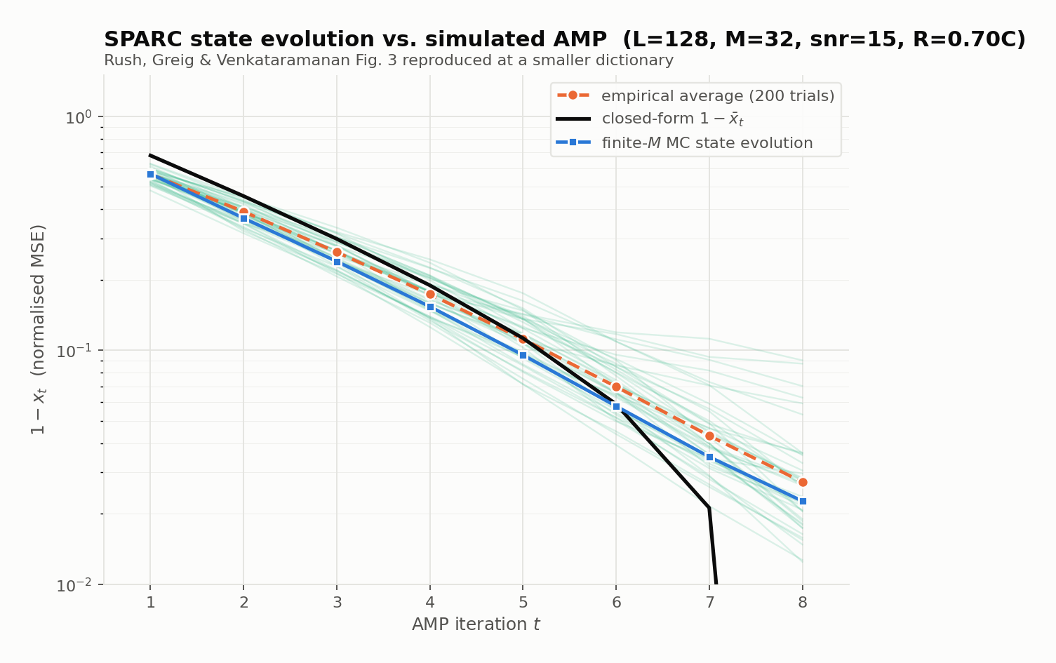

Performance Guarantees

The asymptotic guarantee established by this analysis is stated precisely in Rush, Greig, and Venkataramanan’s Theorem 1: for any fixed rate $R < C$, the SPARC ensemble with $M = L^{\mathsf{a}}$, exponentially decaying power allocation, and AMP run for exactly $T^*$ steps has a section error rate that converges to zero almost surely as $n \to \infty$. The quantifier order is the strong form of the claim: the result holds for every fixed rate below capacity, not merely for rates within a fixed gap of it. This places SPARCs alongside Arıkan’s unconditional theorem for polar codes and the performance that Richardson and Urbanke’s optimized irregular LDPC ensembles approach only empirically, reached here through entirely different mathematics: statistical estimation theory rather than martingale arguments or graph combinatorics.

A vanishing section error rate does not immediately imply a vanishing message error probability, since a single incorrect section out of $L$ still corrupts the decoded message. The resolution repeats a structural pattern already established in this series: an outer Reed-Solomon code of rate $1 - 2\epsilon$ over an alphabet of size $M$ is concatenated with the SPARC, so that each RS symbol addresses exactly one section. If the inner SPARC’s section error rate falls below $\epsilon$, the outer RS code corrects it exactly, and the overall rate becomes $R(1-2\epsilon) \to R$ as $\epsilon \to 0$. This is structurally the same construction as polar’s CRC-aided SCL: an inner soft, message-passing-decoded code is paired with an outer algebraic code whose sole function is to correct whatever residual errors the inner decoder cannot eliminate on its own. Two entirely different inner decoders, softmax denoising and successive-cancellation list decoding, each required an algebraic outer code of this kind to convert a high-probability guarantee into a provable one.

The theorem also has a notable limitation. Unlike Barron and Joseph’s earlier least-squares result, which provides an explicit error exponent decaying as $\exp(-c \cdot n/(\log B)^2)$ for a rate gap $\Delta = C - R$, Theorem 1 establishes convergence to zero without specifying a rate of decay. This closely mirrors the situation for turbo codes earlier in this series: a union bound identifies the location of the error floor, but the rate at which the waterfall itself descends is a separate and harder question, answered here, as there, empirically rather than analytically.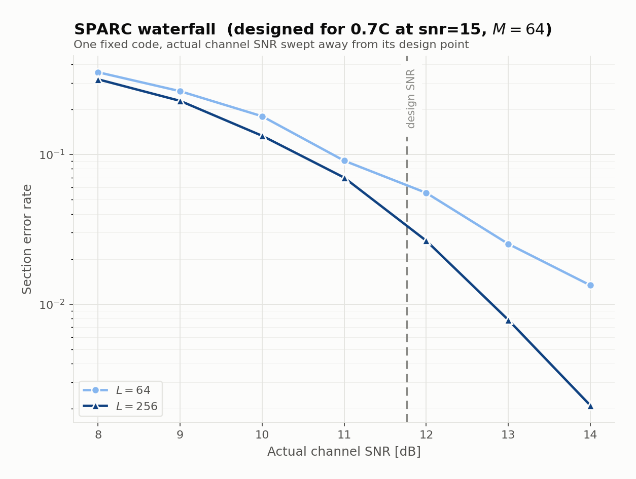

Practical Design Considerations

The exponentially decaying allocation for which Theorem 1 is proved is not the allocation that performs best at the finite block lengths used in practice. The paper’s refinement introduces two parameters, $(\mathsf{a}, f)$: exponential decay, $P_\ell \propto 2^{-\mathsf{a} \cdot 2C\ell/L}$, up to section $fL$, followed by a flat allocation over the remaining $(1-f)L$ sections. Tuning these parameters exposes a three-way trade-off. Insufficient initial power ($\mathsf{a}$ too small) prevents the first sections from clearing the decoding threshold, so the bootstrapping process never begins. Excessive initial power ($\mathsf{a}$ near the pure-exponential value of 1) performs well near capacity but is wasteful further from it, since power removed from the tail sections leaves them undecodable even after the head has successfully bootstrapped. Flattening the tail ($f < 1$) provides the weakest sections with a power floor rather than allowing the allocation to decay to zero, directly analogous to the way irregular LDPC’s stability condition caps rather than eliminates degree-2 variable nodes: a minimum floor of reliability is necessary throughout the code, not only where the allocation happens to be generous. Tuning $(\mathsf{a}, f)$ under a fixed power budget is the same design problem as choosing an LDPC degree distribution or a turbo interleaver length: a shared resource, distributed unevenly, to exploit a bootstrapping mechanism that functions only if the distribution is correct.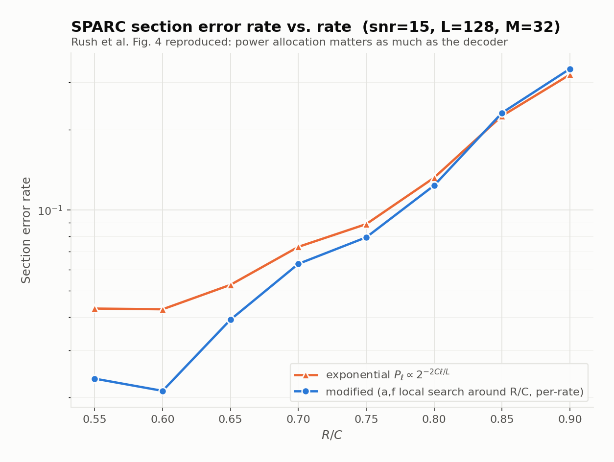

A second practical bottleneck is computational rather than statistical. A Gaussian $A$ requires $O(nN)$ time and $O(nN)$ memory per AMP iteration, since every matrix-vector product is dense and the full matrix must be stored. Both costs are eliminated by constructing $A$ from rows of a Hadamard matrix instead of drawing it i.i.d. Gaussian: define $H_0 = 1$ recursively, with $H_m$ the $2 \times 2$ block matrix having $H_{m-1}$ in the top-left, top-right, and bottom-left blocks and $-H_{m-1}$ in the bottom-right, then select $n$ rows of $H_m$ uniformly at random (for $N = ML = 2^m$) and scale by $1/\sqrt{n}$. Because $H_m$ is exactly the kernel of the fast Walsh-Hadamard transform, both $A\beta^t$ and $A^\top z^t$ can be computed in $O(N \log N)$ time, and $A$ itself never needs to be stored; only $O(N)$ vectors are held in memory at any point.

This result is worth highlighting explicitly: it is the same butterfly, recursive-doubling structure that gives polar encoding and successive-cancellation decoding their $O(N \log N)$ complexity, reappearing here as the mechanism that resolves SPARC decoding’s $O(nN)$ dense-matrix bottleneck. Polar codes and SPARCs share almost no design principles: one is a deterministic recursive channel transform constructed to avoid randomness entirely, the other a dense random Gaussian regression problem constructed to exploit it. Yet the moment each requires moving $N$-dimensional data through a structured linear map efficiently, both converge on the identical fast transform. This is the second instance in this series of two families, developed for unrelated reasons, converging on the same algorithmic tool, suggesting that the transform reflects a more fundamental computational structure than either paper’s original motivation suggests.

Check Yourself

1. Why does building the design matrix $A$ dense, rather than sparse, make sense for SPARCs when every other family in this series worked hard to keep its structure sparse?
2. What does the Onsager term correct for, and which two other decoders’ design principles is it most directly analogous to?
3. A SPARC uses flat power allocation with a strong, efficient (non-AMP) decoder. What limitation does it still hit, and why doesn’t a better decoder fix it?
4. Why is $x_{t+1}$ described as a “power-weighted fraction of correctly decoded sections,” and what identity makes that reading precise?
5. What does a Hadamard design matrix buy an AMP decoder, and what is given up to get it?
6. Theorem 1 proves the section error rate goes to zero for every $R < C$. Why is that not automatically a proof that the message error probability also goes to zero, and what closes the gap?

Answers

1. SPARCs get their tractability from a different asymptotic tool than the rest of the series: state evolution, which is exact precisely because $A$ is dense with i.i.d. Gaussian entries; that density is what makes the Gaussian approximation of the test statistic $s^t$ rigorous. LDPC, turbo, and polar instead rely on local graph algorithms (belief propagation, BCJR, successive cancellation) that are only exact on trees, so for them a dense graph would destroy tractability rather than create it.

2. It corrects a first-order self-interaction bias so that the test statistic $s^t$ stays asymptotically clean signal plus independent Gaussian noise. It plays the same role as LDPC belief propagation’s exclusion of a variable’s own previous message in the check-to-variable update, and as turbo decoding’s extrinsic-information subtraction: all three exist to stop a decoder from being fooled by an echo of its own earlier output.

3. The achievable rate is capped at $R_0 = \tfrac12 P/(P+\sigma^2) < C$, a hard ceiling created by the power allocation itself rather than by any weakness in the decoder. No decoder improvement removes this cap without also changing how power is spread across sections.

4. Because $x_{t+1} = \frac{1}{nP}\mathbb{E}[\beta^\top \beta^{t+1}]$, and each term $\beta_i \beta_i^{t+1}$ is appreciable only when both factors are large, which happens essentially only at the true nonzero index of each section, weighted by that section’s power $P_\ell$. The identity that makes this exact is the state-evolution definition itself, which equates this power-weighted inner product with one minus the (also power-normalized) mean-squared error.

5. It reduces AMP’s per-iteration cost from $O(nN)$ time and $O(nN)$ memory (Gaussian $A$, which must be stored explicitly) to $O(N \log N)$ time and $O(N)$ memory, via the fast Walsh-Hadamard transform, with $A$ never stored at all. The cost is losing the freedom to draw an arbitrary Gaussian ensemble; you are restricted to random row-subsets of a fixed Hadamard structure, though empirically performance stays close to the Gaussian case.

6. A vanishing section error rate still permits a small but nonzero fraction of wrong sections, and even a single wrong section corrupts the decoded message. Concatenating an outer Reed-Solomon code (rate $1-2\epsilon$, alphabet size $M$) closes the gap: if the SPARC’s section error rate falls below $\epsilon$, the RS code corrects it exactly, driving the message error probability to zero as well, the same inner-code, outer-code division of labor as polar’s CRC-aided SCL.

Where This Leaves Us

This page has traced four connective threads through the series. The exclusion principle appeared for a fourth time: LDPC belief propagation excluding a variable’s own message, turbo decoding subtracting the channel and a priori terms to construct an extrinsic LLR, polar SCL’s ordering requirement between killing and cloning paths, and now AMP’s Onsager term, all performing the same function of preventing self-reinforcement, here transplanted from a sparse combinatorial graph to a dense continuous one. State evolution proved to be density evolution’s counterpart for dense graphs, applying the same technique of collapsing an intractably large state into a scalar recursion, computed once offline before decoding begins, regardless of whether the underlying structure is a sparse Tanner graph or a dense Gaussian matrix. The pattern of an outer code correcting the residual errors of an inner soft decoder recurred for a second time, with an outer Reed-Solomon code performing for AMP’s section errors the same role that an outer CRC performs for polar’s SCL failures. And the fast Hadamard transform recurred for a second time as well, the same recursive-doubling structure rescuing two code families, developed for unrelated reasons, from the same computational bottleneck.

Taken together, these four threads bring the shape of the whole series into focus. Turbo, LDPC, and polar codes each built distinct, purpose-specific structure, and the analytical and algorithmic tools required to decode that structure converged independently on a common set of ideas: exclusion principles, threshold recursions, outer-code correction, and fast structured transforms. SPARCs reach the same set of tools from the opposite direction, starting from Shannon’s original unstructured randomness and adding back only the minimum structure an efficient decoder requires. That two such different approaches, one imposing structure on a graph, the other withholding structure from a matrix, converge on the same small set of ideas is not incidental; it is the substance of the answer to this series’ opening question. Shannon’s 1948 existence proof and the sixty years of engineering that followed it constitute two distinct routes to the same set of results, and the tools that emerge, extrinsic exclusion, offline threshold computation, outer algebraic correction, fast structured transforms, are largely independent of which route is taken. Readers interested in pursuing this thread further may consult Donoho, Maleki, and Montanari’s 2009 paper, which first derived the Onsager correction for the more general compressed-sensing problem, and the application of SPARCs to unsourced random access, which repurposes the same machinery for an entirely different communication problem involving many users and no identities, a further indication that the ideas developed in this series extend well beyond any single code.