Multiprocessors & SoC

Phase 6 worked out how a single CPU juggles several tasks at once: priorities, scheduling policies, IPC. This phase asks a question that sits one level above all of that: what if the right answer, for a given embedded product, isn’t a single (however well-scheduled) CPU at all? Wolf’s chapter on multiprocessors makes the case that most real embedded systems are built from several processing elements working together, and that the reasons for reaching for more than one processor go well beyond simply needing more raw speed.

Why Multiprocessors: Cost, Real Time, and Power

The first argument is economic. Processor purchase price is a nonlinear function of performance: the fastest chips are rare, so they command a disproportionate market price. That means splitting an application across several cheaper, slower processors is often more cost-effective than buying one expensive fast one, even once you account for the extra engineering effort of partitioning the system across them. It’s a direct generalization of the predictability-versus-throughput trade-off theme from earlier phases into a cost dimension.

The second argument is about real-time performance. Segregating a time-critical process onto its own dedicated processing element avoids the scheduling-overhead tax from Phase 6 entirely for that process. Because that overhead is paid at the same nonlinear cost-per-performance rate as everything else, avoiding it by adding a second cheap processing element can be much cheaper than buying enough single-CPU headroom to absorb the overhead instead.

The third argument is power, and Wolf makes it with a genuinely striking number. Performance scales roughly linearly with supply voltage, but power scales with $V^2$: the CMOS power law from Phase 3. So several slower processors running at lower voltage can do the same total work for less power than one fast processor running at high voltage. Austin et al.’s measured gap is worth remembering as a concrete figure: battery power delivers roughly 75 mW, while a desktop-class processor draws on the order of 1000 times that. It’s a gap that no amount of tweaking a single processor’s architecture or software can close, and it’s the structural reason battery-powered embedded devices lean on multiprocessing rather than simply chasing a faster uniprocessor.

Accelerators: The CPU’s Smart Peripheral

Wolf’s central worked example of custom multiprocessing is the accelerator, and it’s worth keeping precise how an accelerator differs from both a CPU and a co-processor. A co-processor, from Phase 3, is wired into the CPU’s internals and executes reserved opcodes as part of the instruction stream itself. An accelerator, by contrast, sits on the CPU bus like any other I/O device, controlled through data and control registers via a programming-model interface: functionally it’s closer to a smart peripheral than to an extension of the CPU’s own instruction set. Both, in the end, just do the computation the specification requires; from a pure functionality standpoint it doesn’t matter whether the work happens on a programmable CPU or in hardwired logic, only whether the result meets the system’s speed, power, and cost targets.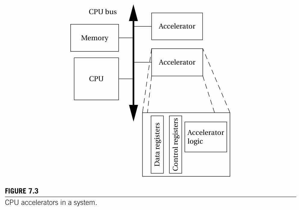

Designing an accelerator is a hardware/software co-design task, not just “write some hardware.” Given an algorithm, usually starting life as a high-level-language description, you have to translate it into a hardware design, build the CPU-bus interface (registers, possibly DMA address-generation logic, shared-memory synchronization), and write the CPU-side driver code that hands off work and retrieves results. All three parts have to work together for the accelerator to actually pay off.

Internally, an accelerator’s own registers and prefetching reduce round-trips to main memory, the same locality principle a cache exploits. Read/write units let it stream data in and out via DMA independently of its core computation, overlapping data movement with computation in exactly the pattern already familiar from Phase 4 and Phase 5.

That independence is also where a genuinely new problem shows up: cache coherence with an independent writer. If the CPU has cached location S, and the accelerator then writes S directly in main memory, a subsequent CPU read of S may return the CPU’s own stale cached value rather than the accelerator’s update. This is the multiprocessor-scale instance of the “which copy is authoritative” problem caches always create, now with a writer that the CPU’s own cache-consistency logic simply doesn’t know about. The fixes mirror what’s already familiar from earlier phases: explicit cache-invalidation instructions, evicting the line by reading an aliased address, or, better, CPU and bus hardware built for multiprocessing that lets other processing elements signal the cache updates they require directly.

Synchronizing the CPU and the accelerator reuses Phase 6’s IPC machinery directly. A simple write-buffer, start, wait, read-results protocol acts as an implicit semaphore, mediated through the accelerator’s status registers. If the CPU and accelerator need concurrent access to the same block of memory, the accelerator itself needs a test-and-set capability on the bus, exactly like inter-process shared-memory synchronization on a single CPU.

Measuring Whether an Accelerator Actually Helps

Before any power or cost argument matters, there’s a prior question: does the accelerator actually speed the system up? In the simple, non-overlapped case, an accelerator’s execution time is just its data movement plus its core compute time:

$$t_{accel} = t_{in} + t_x + t_{out}$$

From that, the speedup of replacing a software kernel with an accelerator invoked $n$ times works out to

$$S = \frac{n \cdot t_{CPU}}{n \cdot t_x + t_{in} + t_{out}}$$

where $t_{CPU}$ is the equivalent software execution time, obtainable with Phase 5’s performance-analysis techniques. Note that $t_{in}$ and $t_{out}$ don’t scale with $n$ if the data stays resident, which is exactly why amortizing that overhead over many invocations increases the realized speedup. The data-movement overhead here isn’t a rounding error: an accelerator that’s fast at its core computation but slow to get data in and out can easily end up a net loss once that overhead is counted. It’s the same “count the whole path, not just the fast part” lesson as Phase 5’s execution-time analysis, now applied across a hardware/software boundary instead of within a single CPU’s pipeline.

How the CPU drives the accelerator also changes how system-level speedup has to be computed. In single-threaded use, the CPU simply blocks and waits for the accelerator, so there’s one execution path and the system speedup is just the accelerator’s own speedup $S$. In multithreaded use, the CPU does other useful work while the accelerator runs, so system time is set by the longest path through the now-branching execution graph: speeding up the accelerated function only helps system-level time if that function’s path was actually the critical, longest one. It’s a textbook Amdahl’s-law-style lesson, but made concrete and graph-based rather than left as an abstract formula.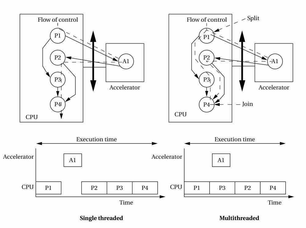

Scheduling, Allocation, and Pipelining Across Processors

Once a system has more than one processor, scheduling and allocation stop being independently optimizable choices. Wolf’s worked two-processor example makes this concrete: a “natural” allocation that follows precedence order (tasks P1 and P2 on processor M1, P3 on M2) leaves M2 idle while it waits on data from M1. A different allocation that looks less clean on paper (P1 on M1, P2 and P3 both on M2) actually runs faster, because it lets P1 and P2 execute concurrently. The obvious, intuitive way to partition a task graph onto hardware is not automatically the fastest one.

Overlapping computation and communication pushes the same idea further: splitting one large message transfer into smaller pieces lets a downstream task start consuming the first piece before the rest has even arrived. It’s the streaming and pipelining idea from Phases 4 and 5, applied to inter-processor communication instead of a single data path. Wolf’s worked example cuts total schedule length from 15 steps to 12 purely by restructuring when data is sent, without changing any of the computation itself.

That restructuring choice generalizes into a broader point about buffering and pipeline scheduling: they affect latency, not just throughput. Processing all of stage A, then all of stage B, then all of stage C in batch delays the first real output until $2n+1$ steps in. Interleaving the stages instead, so that A[0] feeds B[0] feeds C[0] before A[1] even starts, produces the first output after just 3 steps and a new output every 3 steps thereafter. Both schedules do the same total work, but their latency profiles are dramatically different. The general lesson for any multi-stage pipeline is that batch processing optimizes for simplicity while pipelined, interleaved processing optimizes for latency, and which one an application actually needs depends on the application.

Finally, when data has to move across several memories rather than just within one, both delay and energy compound. Multi-hop copying between different memories is gated by the slowest link along the path (source memory, bus, or destination memory), and it costs the sum of every component’s energy along that same path. It’s a direct generalization of Phase 4’s single-bus bandwidth analysis to a system with several hops instead of one.

Convergent Architecture in Consumer Electronics

Wolf closes the chapter with a case-study survey of consumer electronics, phones, CD and DVD players, audio players, digital cameras, and despite how different these products look on the outside, they converge on the same handful of architectural building blocks: a general-purpose control CPU, one or more DSPs or accelerators for the actual media codec work, and shared, DMA-based memory access tying them together. The accelerator and multiprocessor patterns discussed above aren’t a theoretical exercise; they’re literally how real consumer SoCs get built, and the same shape recurs across chapter after chapter of case studies.

Closing the Loop, and Looking Toward Networks

Almost everything in this phase is a payoff of earlier phases rather than a truly standalone idea. The cost/performance nonlinearity argument depends on Phase 2’s ISA-versus-realization framing; the power argument depends on Phase 3’s CMOS $V^2$ power law; the accelerator-as-smart-peripheral framing depends on Phase 3’s co-processor and I/O-device distinctions; the cache-coherence problem is Phase 3’s cache material colliding with a second, independent writer; the synchronization mechanisms are lifted directly from Phase 6’s IPC section; and the speedup, scheduling, and allocation analysis is Phase 5’s execution-time-and-path-analysis machinery applied across a hardware/software boundary instead of within one CPU. The one genuinely new idea this phase adds on top of all that is that the nonlinear cost/performance curve is itself a first-class design constraint, on equal footing with the timing and power constraints that have driven every decision so far. Sometimes the “obviously right” architecture, one fast CPU, is wrong purely on a dollars-per-unit-performance basis, independent of whether a single CPU could technically do the job.

It’s also worth flagging that this chapter’s treatment of cache coherence, invalidate the line or design multiprocessing-aware hardware, is a starting point rather than the full story; modern SoCs handle this at scale with coherent interconnects and snooping protocols that go well beyond what a single accelerator’s status registers can express. That points naturally at the next phase: everything here assumed processing elements sitting together on one board or one chip, coordinating over a shared bus. Phase 8 stretches the same underlying problems, data-movement overhead, synchronization, and scheduling across branching execution paths, across an actual network, where the links are slower, less predictable, and no longer guaranteed to be there at all.