Verification & Correctness (Formal Methods)

Phase 8 was about getting distributed embedded nodes to agree with each other over an unreliable network; this phase asks a more basic question about any of those nodes taken alone: how do you know a design is actually correct, rather than merely tested and not-yet-observed-to-fail? It is also, in a real sense, the payoff for Phase 1‘s formal apparatus. The computation trees, behaviors, traces, and nondeterminism introduced there to describe what a state machine can do turn out to be exactly the machinery this phase needs to prove things about what a state machine can do. Four chapters of Lee and Seshia (LS) form one continuous arc: specify precisely what correct means (Ch.13), decide when one model can safely stand in for another (Ch.14), turn that specification into an algorithm that checks compliance (Ch.15), and finally extend the whole discipline from yes/no properties to actual quantities like execution time (Ch.16).

Specifying Correctness: Invariants and Temporal Logic

The starting problem is that natural-language requirements are systematically ambiguous. LS’s own example is a real space-agency standard for the SpaceWire protocol, whose English text never says when (“immediately”? “eventually”?) a particular state transition has to happen, even though the intended answer (the next clock tick) mattered a great deal to anyone implementing it. The chapter’s guiding line is worth keeping close: a design without a specification cannot be right or wrong, it can only be surprising.

The simplest and most common shape a specification takes is an invariant: a property that is true in the initial state and preserved by every reaction thereafter. Invariants span an enormous range, from “no pedestrian crossing while the light is green” (the traffic light example from Phase 1) to “never dereference a null pointer” to “no thread deadlocks.” A postcondition constraining a function’s output range, as in LS’s real Paparazzi UAV altitude-control example, is just a special case of an invariant too.

LTL (Linear Temporal Logic) is what lets you say more than plain invariants. It extends ordinary propositional logic (atomic propositions like x=present, combined with ∧, ∨, ¬, ⇒) from statements about one reaction to statements about entire traces, via four temporal operators. For a trace $q_0, q_1, q_2, \ldots$:

$$\mathbf{G}\varphi \text{ holds} \iff \forall j\ge 0,\ \varphi \text{ holds at } q_j, q_{j+1}, \ldots$$ $$\mathbf{F}\varphi \text{ holds} \iff \exists j\ge 0,\ \varphi \text{ holds at } q_j, q_{j+1}, \ldots$$ $$\mathbf{X}\varphi \text{ holds for } q_0,q_1,\ldots \iff \varphi \text{ holds for } q_1, q_2, \ldots$$

In words: G φ (“globally”) means φ holds at every point in the trace, which is exactly an invariant when φ is a plain proposition; F φ (“eventually”) means φ holds at some point; X φ (“next”) means φ holds starting at the very next reaction; and φ₁ U φ₂ (“until”) means φ₁ holds continuously up to the point where φ₂ becomes true, which must eventually happen. An LTL formula “holds for a machine” only if it holds for every possible trace, and proving that is generally much harder than finding one counterexample trace where it fails. That asymmetry, easy to refute, hard to prove, is the same shape as the interchange-argument proofs used for scheduling optimality in Phase 6.

The real expressive power comes from composing these operators. $\mathbf{G}(p\Rightarrow \mathbf{F}q)$ is a request-response pattern (“every request eventually gets a response”); $\mathbf{GF}p$ says “p happens infinitely often,” a fairness property; $\mathbf{FG}p$ says “eventually p holds forever,” a steady-state property. These three composite shapes recur constantly enough that they’re worth memorizing as idioms rather than re-deriving each time.

That last pair also points at the fundamental property taxonomy: safety (“nothing bad ever happens,” violated by some finite bad prefix, of which any invariant is the paradigm case) versus liveness (“something good eventually happens,” which no finite trace can refute, only an infinite one can). The split matters practically because it predicts which verification technique applies: Ch.15’s reachability analysis handles safety properties (G p) directly, while liveness needs the heavier Büchi-automaton machinery described below. Bounded liveness (a time-bounded “eventually,” such as “the ISR runs within 100 cycles”) is secretly a safety property in disguise, since a violation still shows up as a finite bad prefix; unbounded liveness is not, and LTL’s X operator can only express a limited, bounded form of it.

Equivalence and Refinement: When Can One Model Stand In for Another?

Chapter 14’s motivating question is concrete: given a specification model $A$ and a candidate implementation or replacement model $B$, when is it safe to substitute $B$ for $A$? LS builds a hierarchy of increasingly strong answers, and it helps to hold the whole ladder in view before the details: type refinement is the weakest relation, language refinement is stronger, simulation stronger still, and bisimulation strongest of all, each successive relation strictly harder to satisfy than the last.

Type refinement checks only port existence and data types. $B$ type-refines $A$ if all four of the following hold:

$$P_B \subseteq P_A, \qquad Q_A \subseteq Q_B, \qquad \forall p \in P_B,\ V_p \subseteq V_p', \qquad \forall q \in Q_A,\ V_q' \subseteq V_q$$

That is: $B$‘s input ports are a subset of $A$‘s (safe, since $B$ can simply ignore inputs it doesn’t need), $B$‘s output ports are a superset of $A$‘s (safe, since the environment can ignore extra outputs), $B$ accepts every input value $A$ would have accepted, and every output $B$ produces is acceptable wherever $A$‘s outputs were acceptable. Passing this check only guarantees the absence of type-system errors from the substitution; it says nothing about actual behavior.

Language equivalence and containment go further, comparing the actual sets of input/output sequences, that is, the machine’s language $L(M)$, straight out of Chapter 3’s behavior and trace definitions from Phase 1. $A$ is a language refinement of $B$ if $L(A) \subseteq L(B)$: every behavior $A$ can produce, $B$ could also have produced, so $A$ is safe to substitute wherever $B$ was acceptable. Regular languages, regular expressions, and the Kleene star are the classical machinery for describing these sequence sets compactly, and Büchi automata extend the idea to infinite executions, accepting a trace when it visits an accepting state infinitely often. That acceptance condition is exactly the mechanism Ch.15 reuses for liveness model checking.

Language containment turns out not to be enough on its own. Two nondeterministic machines can be language-equivalent, capable of producing exactly the same behaviors, yet observably differ once you can no longer see the future. LS’s worked example (Figure 14.3) has a machine $M_1$ that can always “predict and dodge” $M_2$‘s nondeterministic choices, exposing outputs $M_2$ can never match, even though the two machines’ overall languages are identical. This is the chapter’s central insight: capability to produce the same behaviors is not the same thing as being safe to swap in real time, once nondeterminism, and the resulting inability to see the future, is in play.

Simulation is the fix. Picture a matching game: $M_2$ moves first each round, making any nondeterministic choice it likes, and $M_1$ must respond with a move producing the same output, using only present information, no peeking ahead. $M_1$ simulates $M_2$ if it can always win this game. Formally, $M_1$ simulates $M_2$ if there exists a simulation relation $S \subseteq States_2 \times States_1$ such that $(s_0^2, s_0^1) \in S$, and for every pair already in $S$ and every possible move $M_2$ could make, $M_1$ has a matching move landing back in $S$ with the same output:

$$(s_2,s_1)\in S \implies \forall x,\ \forall (s_2', y)\in possibleUpdates_2(s_2,x),\ \exists (s_1', y)\in possibleUpdates_1(s_1,x) \text{ s.t. } (s_2',s_1')\in S$$

Such a relation records every reachable pairing of states across all possible plays. Simulation is transitive, which lets you chain simulations across a whole design-refinement sequence, but it is generally not unique: multiple valid simulation relations can exist when the simulating machine has its own nondeterministic freedom in how it matches. Crucially, $M_1$ simulates $M_2$ implies $L(M_2) \subseteq L(M_1)$, but not the other way around; language containment alone does not imply simulation, which is precisely the gap the dodging example above exposes.

Bisimulation is the strongest relation in the hierarchy: the same matching game, but played symmetrically, so either machine may move first each round and the other must always match. $M_1$ and $M_2$ are bisimilar if and only if each simulates the other and the game works with either one moving first; simulating each other one-directionally is not by itself sufficient. LS’s Figure 14.5 gives a pair of machines that simulate each other yet are not bisimilar, because alternating who moves first each round can still expose an unmatched move. Bisimilar machines are truly indistinguishable from any environment’s perspective, the gold-standard equivalence in the hierarchy.

The practical payoff of building this whole ladder is that it justifies model reduction and abstraction in verification (Ch.15): if you can show that a small abstract model bisimulates, or is properly simulated by, a large concrete one, then any property proven on the small model transfers to the large one for free.

Reachability Analysis and Model Checking

Model checking is the algorithmic version of all of the above: deciding whether a finite-state system satisfies an LTL specification. The idea earned Clarke, Emerson, and Sifakis the 2007 Turing Award, a good indicator of how foundational it is to the field.

Verification needs a closed system, one with no free inputs, to have well-defined behavior to check against. So in practice you compose the system under test $S$ with an explicit model of its environment $E$, using the composition operators from Chapters 5 and 6 covered in Phase 1, to obtain a closed verification model $M$, and then check $M$ against the property $\Phi$. A “NO” verdict comes with a counterexample, an error trace, which is genuinely one of formal verification’s best practical features: it hands you a concrete, debuggable witness rather than just an abstract “it’s broken.”

Reachability analysis handles the $\mathbf{G} p$ case directly. View the state space as a directed graph (the state graph): $M \models \mathbf{G} p$ iff every reachable state satisfies $p$. Explicit-state model checking does a depth-first search from the initial state, building the graph on the fly and tracking a visited set $R$. It is conceptually simple and terminates for any finite-state $M$, but its cost is proportional to the actual number of states, which is where the state-explosion problem bites. Composing $k$ subsystems with $n_1, \ldots, n_k$ states each yields a state space of size

$$|States(M_1 \| \cdots \| M_k)| = \prod_{i=1}^k n_i$$

growing exponentially in the number of composed components: one hundred boolean state variables already give $2^{100}$ states, utterly beyond explicit enumeration.

Symbolic model checking is the standard fix: represent sets of states as propositional-logic formulas rather than enumerating them individually, and compute reachability via image computation (one symbolic “apply the transition relation to this whole set” step) plus set union and emptiness checks, instead of one-state-at-a-time depth-first search. LS’s traffic-light example makes the payoff concrete: the reachable set after $k$ steps can be a compact formula like "$0 < count \le 60$" standing in for dozens of individual states. The compression can be dramatic, though in the worst case symbolic representations can still blow up.

Abstraction goes further still: verify a simpler model that has more behaviors than the real system (a sound over-approximation) but is small enough to check quickly. Localization reduction, hiding or freewheeling state variables irrelevant to the property being checked, is the simplest form of this. LS’s traffic-light example collapses 188 states down to 4 by hiding the count variable entirely, since the safety property in question doesn’t depend on it. The general principle is that which details you can safely omit depends entirely on which property you’re checking; there is no one universal “the small model,” only the smallest model sufficient for this particular proof obligation.

CEGAR (CounterExample-Guided Abstraction Refinement) automates the abstraction-picking problem itself: start by hiding almost everything and model-check the crude abstraction. If it passes, so does the real system, since the abstraction only has more behaviors than the concrete one. If it fails, check whether the counterexample is real or an artifact of over-abstraction; if it’s an artifact, add back just enough hidden detail to rule it out, and repeat. It is a genuinely elegant iterative-refinement loop, and it is the basis of real industrial tools such as Microsoft’s SLAM.

Liveness properties need more machinery than plain reachability provides. $\mathbf{F} p$ can be partially checked via $\neg \mathbf{G} \neg p$: if $\mathbf{G} \neg p$ holds, then $\mathbf{F} p$ definitely fails everywhere, but a “NO” answer there only witnesses one trace where $\mathbf{F} p$ holds, not a proof that it holds for all traces. The general LTL model-checking approach represents $\neg \Phi$ as a Büchi automaton $B$, composes it with the system $M$, and checks whether the product $M \otimes B$ can visit one of $B$‘s accepting states infinitely often, forming an acceptance cycle. If it can, $M$ violates $\Phi$; if not, $M$ satisfies it. Nested DFS, used in the real SPIN model checker, solves this efficiently: one depth-first search finds a path to an accepting state, and a second depth-first search launched from there checks whether that state can reach itself again, forming a cycle. It is worth keeping $\mathbf{GF}p$ and $\mathbf{FG}p$ straight, since they are easy to conflate despite being opposite in shape: $\mathbf{GF}p$ (“p infinitely often,” a fairness property, such as “the light turns green infinitely often”) versus $\mathbf{FG}p$ (“eventually p holds forever,” a steady-state property, such as “the robot eventually reaches its target room and stays”). The negation of one is, up to a $p$/$\neg p$ swap, literally the automaton for the other.

Quantitative Analysis: From Yes-or-No to How Much

Chapter 16 reframes the verification question from yes/no to how much: instead of asking whether a system satisfies property $\Phi$, ask what the value of a quantity $q = f_P(x, w)$ is, a function of program inputs $x$ and environment parameters $w$ (such as cache state). There are three standard framings: extreme-case analysis (worst-case or best-case execution time, the maximum or minimum of $q$ over all $x, w$), threshold analysis (is $q \le T$ always, often easier than computing the exact extreme value since you only need to prove a bound, not find the tight one), and average-case analysis (the expected value of $q$ under assumed input and environment distributions, the right framing for energy and power, where the worst case is usually far too pessimistic to be useful).

The unit of analysis is, once again, programs as graphs: a basic block (single-entry, single-exit straight-line code, the same concept as Chapter 5’s CDFG from Phase 5, now called a control-flow graph, or CFG) with call and return edges extending it across function boundaries, or with non-recursive calls simply inlined to avoid needing those edges at all.

Computing worst-case execution time (WCET) is hard for four distinct and compounding reasons. Loop bounds are undecidable in general, since the problem reduces to the halting problem, but provable in practice via a ranking function, or progress measure: LS’s worked example is a shift register whose bit count strictly decreases each iteration, proving termination within 32 steps, the same well-founded-descent argument used to prove any loop terminates. Path space is exponential: a nested loop with $n$ independent branch points inside has up to $2^n$ distinct paths, and LS’s own example is a 100x100 array loop with $2^{10000}$ paths, though the IPET optimization below sidesteps ever having to enumerate them. Path feasibility is a separate problem, since not every syntactic path through the graph is actually executable; LS’s Paparazzi example has two mutually exclusive clamp conditions that can’t both be true, ruling out 2 of 4 inner-branch combinations, and checking feasibility in general is NP-hard, reducing to SAT. And the memory hierarchy can swing execution time by roughly 100x for a seemingly tiny change: LS’s dot-product example changes an array’s size from 2 to 8 and flips every access from a guaranteed cache hit to a guaranteed cache miss, purely because of cache-set aliasing, directly reusing the cache-conflict material from Phase 3 and showing it has first-order impact on timing predictability, not just average throughput.

IPET, the Implicit Path Enumeration Technique, is the chapter’s centerpiece, and it is worth understanding structurally even without memorizing the exact constraint syntax. Each basic block $i$‘s execution count $x_i$ becomes a linear-programming variable. Flow constraints enforce unit flow from source to sink and flow conservation at every node, literally network-flow theory borrowed from traffic and circuit analysis, and logical flow constraints add loop bounds and infeasible-path exclusions to rule out invalid combinations. The optimization then maximizes the sum of per-block time bound times execution count, subject to those constraints:

$$\text{WCET} = \max \sum_{i=1}^n w_i x_i \quad \text{s.t.} \quad \underbrace{x_1 = x_n = 1}_{\text{unit flow}}, \quad \underbrace{x_i = \sum_{j\in P_i} d_{ji} = \sum_{j\in S_i} d_{ij}}_{\text{flow conservation}}, \quad \text{+ logical flow constraints}$$

where $w_i$ is the separately-bounded worst-case time for basic block $i$, and the logical flow constraints add loop bounds ($x_i \le$ bound) and infeasible-path exclusions ($\sum d_{i_kj_k} \le k-1$ for a mutually-exclusive edge set). The genuinely clever part is that this finds the WCET-defining execution counts without ever enumerating actual paths, sidestepping the exponential-path-space problem entirely via a polynomial-time optimization (or, once integrality constraints are added for infeasible-path exclusion, an NP-hard one that is “usually fine in practice”). It is the same move as Ch.15’s symbolic model checking: characterize the set of valid solutions with constraints instead of enumerating it, a pattern worth recognizing as recurring across the whole phase.

The following control-flow graph is LS’s running example for the whole IPET formulation: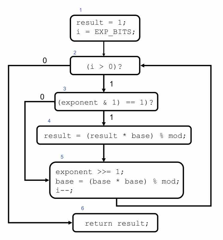

The per-basic-block time bounds $w_i$ that feed into IPET are themselves nontrivial to obtain, and this is where the memory-hierarchy problem feeds back into the optimization: naively summing worst-case per-instruction times is safe but can be roughly 100x too loose if cache hits and misses aren’t distinguished. Real WCET tools either extend the ILP itself with cache-conflict constraints (as in Li and Malik’s work) or use abstract interpretation, a sound over-approximation in the same spirit as Ch.15’s abstraction, to infer invariants about cache and pipeline state at each program point and so obtain tighter, still-safe bounds.

Two further quantitative problems round out the chapter. Stack analysis bounds worst-case stack depth via the call graph, tractable without recursion and considerably harder once interrupts are involved. Energy and power analysis cannot rely on execution time alone, since switching activity depends on the actual data values flowing through the circuit; energy estimation typically resorts to average-case profiling across representative benchmarks rather than a tight worst-case bound.

Characterize, Don’t Enumerate

This is an LS-only phase; Wolf has no equivalent chapters, and it is the clearest demonstration in the whole book of why Phase 1’s formal modeling machinery, state machines, composition, concurrent models of computation, was worth building up front. Every technique covered here, LTL specification, simulation and bisimulation, reachability analysis, WCET’s control-flow-graph optimization, is a direct payoff of that earlier foundation, now turned into algorithms that actually prove things about real systems instead of just modeling them.

A single move recurs across all four chapters: characterize the space of valid behaviors, paths, or states with constraints or relations, and reason about the whole space at once, rather than enumerating it. Propositional formulas stand in for state sets in symbolic model checking; simulation relations stand in for every possible matching-game play; linear-programming constraints stand in for exponentially many program paths in IPET. That “characterize, don’t enumerate” pattern is the single most reusable idea to carry forward from this phase, and it is worth noting that Ch.15’s abstraction and CEGAR loop and Ch.16’s abstract-interpretation timing bounds are really the same underlying idea applied to two different questions, correctness and time, which suggests the two chapters could in principle share a great deal of machinery in a unified analysis framework, even though LS treats them as separate tools. With correctness and timing both covered, the next phase turns to a different kind of property that a design also has to satisfy, not “is it correct” or “is it fast enough,” but “can it be trusted”: Phase 10 takes up security and privacy in embedded systems.